Microeconomice - notes and summary - 4 t/m 6
In every market there are buyers and sellers:
- Consumer theory: A set of decision rules that lead to optimal outcomes for the buyer. A
consumer chooses the optimal bundle of goods and services to maximize utility given her
budget
- Producer theory: A set of decision rules that optimize outcomes forthe seller. A seller
chooses whether and how much to produce to maximize net benefits (profit π)
Chapter 6 - Producer behavior
Why do firms maximize profit?
- They can make rational choices (surviving in the market).
- Self-interest.
- CEO receives bonus that is related to the profit.
Assumptions about a firm’s behavior:
1. The firm produces a single good
2. The firm has already chosen which product to produce
3. Firms minimize costs associated with every level of production
• Necessary condition for profit maximization
4. Only two inputs are used in production: Capital and labor
• Capital: Land, buildings (factories, stores), equipment (machines,trucks)
• Labor: All human resources
5. In the short run, firms can choose the amount of labor but capital is assumed to be fixed
6. Output increases with inputs
7. The firm can employ unlimited capital and labor at fixed prices
8. Capital markets are well functioning (the firm is not budget-constrained)
A firm engages in technologically efficient production (TEP) if it cannot produce its current level of
output Q with fewer inputs, given existing knowledge about technology or if it cannot produce more
with its current levels of inputs, given existing knowledge about technology
Short run = the period of time during which capital cannot be changed. K is fixed. 6 to 12 months.
Long run = the period of time during which all inputs are fully adjustable.
Production in the short run → K is fixed, L is variable.
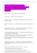
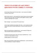
The marginal product of labor (MPL) is the additional output that a
firm can produce using an additional unit of the variable input (L),
holding the other input constant (K fixed).
The MPL increases with the first workers because of specialization. Specialization occurs when
workers develop a particular skill set because they perform a particular task over a period of time.
Specialization is likely to result in increasing returns to scale.
Eventually MPL will fall when L increases with a fixed K → the law of diminishing marginal returns.
The diminishing marginal product of labor is the reduction in extra output obtained from adding
more and more labor. If the amount of capital is held constant, each
additional worker eventually generates less output than the one before.
The same diminishing returns exist for capital when labor is held constant.
,This assumption captures the basic idea of production; a mix of labor and capital is more productive
than capital alone or labor alone.
The MPL can be negative because when more and more workers keep getting added, they will get in
each others way and actually cause output to fall
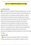
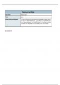
Average product of labor (APL) is total output produced per unit of
the variable input employed (L), holding the other input constant (K).
Production in the long run → K and L are both variable.
Each isoquant shows the possible combinations of labor (L) and capital (K) that produce output (Q).
Isoquants are almost the same as the indifference curves of a consumer:
- The farther away from origin the better.
- Downwards sloping and convex to origin.
- Isoquants do not cross. Such intersections are inconsistent with the requirement that the
firm always produces efficiently.
- The change in input prices does not affect the isoquant.
The shape of the isoquant reveals information about the relationship between inputs:
- Relatively straight isoquants imply that the inputs are relatively substitutable.
o Substitutes: production of electricity from either oil or natural gas.
o Perfect substitutes: Robots and labor.
- Relatively curved isoquants imply that the inputs are relatively complementary.
o Complements: provision of bus services.
o Perfect complements: cabs and drivers.
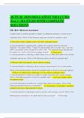
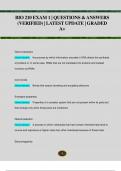
The marginal rate of technical substitution (MRTS) is the rate at which the firm can trade labor for
capital and holding output (Q) constant.
Input on horizontal axis must be on top.
The challenge of producing a specific amount of a particular good as inexpensively as possible is the
firm’s cost-minimalization problem. Cost minimization occurs when MPL / W = MPK / R
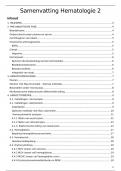
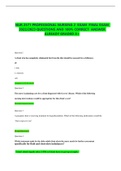
The isocost line is a curve that shows all of the input combinations that yield the same cost (same as
budget line). C = RK + WL → solve for K →
The slope of the isocost line measures how much more units of one input a firm can use if it uses
less units of another input without increasing total cost. According to assumption 7, the slope is
constant. Slope = -(W/R).
, Returns to scale (RTS) refers to the change in output when all outputs are increased in the same
proportion.
A firm achieves an economically efficient point of production (EEP) if it produces a specific amount
of production (Q fixed) at minimum cost or if it maximizes its production (Q) for a given level of total
cost (C fixed). he two constrained optimization problems yield the same optimum.
The firm can choose any of three equivalent approaches to minimize its cost:
- Lowest-isocost rule (pick the bundle where the lowest isocost line touches the isoquant).
- Tangency rule (pick the bundle of inputs where the isoquant is tangent to the isocost line).
- Last-dollar rule (pick the bundle of inputs where the last dollar spent on one input gives as
much extra output as the last dollar spent on any other input).
In every market there are buyers and sellers:
- Consumer theory: A set of decision rules that lead to optimal outcomes for the buyer. A
consumer chooses the optimal bundle of goods and services to maximize utility given her
budget
- Producer theory: A set of decision rules that optimize outcomes forthe seller. A seller
chooses whether and how much to produce to maximize net benefits (profit π)
Chapter 6 - Producer behavior
Why do firms maximize profit?
- They can make rational choices (surviving in the market).
- Self-interest.
- CEO receives bonus that is related to the profit.
Assumptions about a firm’s behavior:
1. The firm produces a single good
2. The firm has already chosen which product to produce
3. Firms minimize costs associated with every level of production
• Necessary condition for profit maximization
4. Only two inputs are used in production: Capital and labor
• Capital: Land, buildings (factories, stores), equipment (machines,trucks)
• Labor: All human resources
5. In the short run, firms can choose the amount of labor but capital is assumed to be fixed
6. Output increases with inputs
7. The firm can employ unlimited capital and labor at fixed prices
8. Capital markets are well functioning (the firm is not budget-constrained)
A firm engages in technologically efficient production (TEP) if it cannot produce its current level of
output Q with fewer inputs, given existing knowledge about technology or if it cannot produce more
with its current levels of inputs, given existing knowledge about technology
Short run = the period of time during which capital cannot be changed. K is fixed. 6 to 12 months.
Long run = the period of time during which all inputs are fully adjustable.
Production in the short run → K is fixed, L is variable.
The marginal product of labor (MPL) is the additional output that a
firm can produce using an additional unit of the variable input (L),
holding the other input constant (K fixed).
The MPL increases with the first workers because of specialization. Specialization occurs when
workers develop a particular skill set because they perform a particular task over a period of time.
Specialization is likely to result in increasing returns to scale.
Eventually MPL will fall when L increases with a fixed K → the law of diminishing marginal returns.
The diminishing marginal product of labor is the reduction in extra output obtained from adding
more and more labor. If the amount of capital is held constant, each
additional worker eventually generates less output than the one before.
The same diminishing returns exist for capital when labor is held constant.
,This assumption captures the basic idea of production; a mix of labor and capital is more productive
than capital alone or labor alone.
The MPL can be negative because when more and more workers keep getting added, they will get in
each others way and actually cause output to fall
Average product of labor (APL) is total output produced per unit of
the variable input employed (L), holding the other input constant (K).
Production in the long run → K and L are both variable.
Each isoquant shows the possible combinations of labor (L) and capital (K) that produce output (Q).
Isoquants are almost the same as the indifference curves of a consumer:
- The farther away from origin the better.
- Downwards sloping and convex to origin.
- Isoquants do not cross. Such intersections are inconsistent with the requirement that the
firm always produces efficiently.
- The change in input prices does not affect the isoquant.
The shape of the isoquant reveals information about the relationship between inputs:
- Relatively straight isoquants imply that the inputs are relatively substitutable.
o Substitutes: production of electricity from either oil or natural gas.
o Perfect substitutes: Robots and labor.
- Relatively curved isoquants imply that the inputs are relatively complementary.
o Complements: provision of bus services.
o Perfect complements: cabs and drivers.
The marginal rate of technical substitution (MRTS) is the rate at which the firm can trade labor for
capital and holding output (Q) constant.
Input on horizontal axis must be on top.
The challenge of producing a specific amount of a particular good as inexpensively as possible is the
firm’s cost-minimalization problem. Cost minimization occurs when MPL / W = MPK / R
The isocost line is a curve that shows all of the input combinations that yield the same cost (same as
budget line). C = RK + WL → solve for K →
The slope of the isocost line measures how much more units of one input a firm can use if it uses
less units of another input without increasing total cost. According to assumption 7, the slope is
constant. Slope = -(W/R).
, Returns to scale (RTS) refers to the change in output when all outputs are increased in the same
proportion.
A firm achieves an economically efficient point of production (EEP) if it produces a specific amount
of production (Q fixed) at minimum cost or if it maximizes its production (Q) for a given level of total
cost (C fixed). he two constrained optimization problems yield the same optimum.
The firm can choose any of three equivalent approaches to minimize its cost:
- Lowest-isocost rule (pick the bundle where the lowest isocost line touches the isoquant).
- Tangency rule (pick the bundle of inputs where the isoquant is tangent to the isocost line).
- Last-dollar rule (pick the bundle of inputs where the last dollar spent on one input gives as
much extra output as the last dollar spent on any other input).