LECTURE NOTES - VI
« FLUID MECHANICS »
Prof. Dr. Atıl BULU
Istanbul Technical University
College of Civil Engineering
Civil Engineering Department
Hydraulics Division
, CHAPTER 6
TWO-DIMENSIONAL IDEAL FLOW
6.1 INTRODUCTION
An ideal fluid is purely hypothetical fluid, which is assumed to have no viscosity and
no compressibility, also, in the case of liquids, no surface tension and vaporization. The study
of flow of such a fluid stems from the eighteenth century hydrodynamics developed by
mathematicians, who, by making the above assumptions regarding the fluid, aimed at
establishing mathematical models for fluid flows. Although the assumptions of ideal flow
appear to be far obtained, the introduction of the boundary layer concept by Prandtl in 1904
enabled the distinction to be made between two regimes of flow: that adjacent to the solid
boundary, in which viscosity effects are predominant and, therefore, the ideal flow treatment
would be erroneous, and that outside the boundary layer, in which viscosity has negligible
effect so that idealized flow conditions may be applied.
The ideal flow theory may also be extended to situations in which fluid viscosity is
very small and velocities are high, since they correspond to very high values of Reynolds
number, at which flows are independent of viscosity. Thus, it is possible to see ideal flow as
that corresponding to an infinitely large Reynolds number and zero viscosity.
6.2. CONTINUITY EQUATION
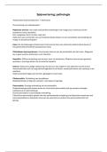
The control volume ABCDEFGH in Fig. 6.1 is taken in the form of a small prism with
sides dx, dy and dz in the x, y and z directions, respectively.
y
B G
A dy
C H x
D E dz
z dx
Fig. 6.1
The mean values of the component velocities in these directions are u, v, and w.
Considering flow in the x direction,
Mass inflow through ABCD in unit time = ρudydz
100 Prof. Dr. Atıl BULU
, In the general case, both specific mass ρ and velocity u will change in the x direction
and so,
⎡ ∂ ( ρu ) ⎤
Mass outflow through EFGH in unit time = ⎢ ρu + dx ⎥ dydz
⎣ ∂x ⎦
Thus,
∂ ( ρu )
Net outflow in unit time in x direction = dxdydz
∂x
Similarly,
∂ ( ρv )
Net outflow in unit time in y direction = dxdydz
∂y
∂( ρw)
Net outflow in unit time in z direction = dxdydz
∂z
Therefore,
⎡ ∂(ρu ) ∂(ρv ) ∂( ρw) ⎤
Total net outflow in unit time = ⎢ + +
∂z ⎥⎦
dxdydz
⎣ ∂x ∂y
Also, since ∂ρ/∂t is the change in specific mass per unit time,
∂ρ
Change of mass in control volume in unit time = − dxdydz
∂t
(the negative sign indicating that a net outflow has been assumed). Then,
Total net outflow in unit time = Change of mass in control volume in unit time
⎡ ∂( ρu ) ∂( ρv ) ∂( ρw) ⎤ ∂ρ
⎢ ∂x + ∂y + ∂z ⎥ dxdydz = − ∂t dxdydz
⎣ ⎦
or
∂ ( ρu ) ∂ ( ρv ) ∂ ( ρw) ∂ρ
+ + =− (6.1)
∂x ∂y ∂z ∂t
Equ. (6.1) holds for every point in a fluid flow whether steady or unsteady, compressible or
incompressible. However, for incompressible flow, the specific mass ρ is constant and the
equation simplifies to
∂u ∂v ∂w
+ + =0 (6.2)
∂x ∂y ∂z
For two-dimensional incompressible flow this will simplify still further to
∂u ∂v
+ =0 (6.3)
∂x ∂y
101 Prof. Dr. Atıl BULU
« FLUID MECHANICS »
Prof. Dr. Atıl BULU
Istanbul Technical University
College of Civil Engineering
Civil Engineering Department
Hydraulics Division
, CHAPTER 6
TWO-DIMENSIONAL IDEAL FLOW
6.1 INTRODUCTION
An ideal fluid is purely hypothetical fluid, which is assumed to have no viscosity and
no compressibility, also, in the case of liquids, no surface tension and vaporization. The study
of flow of such a fluid stems from the eighteenth century hydrodynamics developed by
mathematicians, who, by making the above assumptions regarding the fluid, aimed at
establishing mathematical models for fluid flows. Although the assumptions of ideal flow
appear to be far obtained, the introduction of the boundary layer concept by Prandtl in 1904
enabled the distinction to be made between two regimes of flow: that adjacent to the solid
boundary, in which viscosity effects are predominant and, therefore, the ideal flow treatment
would be erroneous, and that outside the boundary layer, in which viscosity has negligible
effect so that idealized flow conditions may be applied.
The ideal flow theory may also be extended to situations in which fluid viscosity is
very small and velocities are high, since they correspond to very high values of Reynolds
number, at which flows are independent of viscosity. Thus, it is possible to see ideal flow as
that corresponding to an infinitely large Reynolds number and zero viscosity.
6.2. CONTINUITY EQUATION
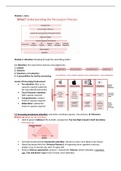
The control volume ABCDEFGH in Fig. 6.1 is taken in the form of a small prism with
sides dx, dy and dz in the x, y and z directions, respectively.
y
B G
A dy
C H x
D E dz
z dx
Fig. 6.1
The mean values of the component velocities in these directions are u, v, and w.
Considering flow in the x direction,
Mass inflow through ABCD in unit time = ρudydz
100 Prof. Dr. Atıl BULU
, In the general case, both specific mass ρ and velocity u will change in the x direction
and so,
⎡ ∂ ( ρu ) ⎤
Mass outflow through EFGH in unit time = ⎢ ρu + dx ⎥ dydz
⎣ ∂x ⎦
Thus,
∂ ( ρu )
Net outflow in unit time in x direction = dxdydz
∂x
Similarly,
∂ ( ρv )
Net outflow in unit time in y direction = dxdydz
∂y
∂( ρw)
Net outflow in unit time in z direction = dxdydz
∂z
Therefore,
⎡ ∂(ρu ) ∂(ρv ) ∂( ρw) ⎤
Total net outflow in unit time = ⎢ + +
∂z ⎥⎦
dxdydz
⎣ ∂x ∂y
Also, since ∂ρ/∂t is the change in specific mass per unit time,
∂ρ
Change of mass in control volume in unit time = − dxdydz
∂t
(the negative sign indicating that a net outflow has been assumed). Then,
Total net outflow in unit time = Change of mass in control volume in unit time
⎡ ∂( ρu ) ∂( ρv ) ∂( ρw) ⎤ ∂ρ
⎢ ∂x + ∂y + ∂z ⎥ dxdydz = − ∂t dxdydz
⎣ ⎦
or
∂ ( ρu ) ∂ ( ρv ) ∂ ( ρw) ∂ρ
+ + =− (6.1)
∂x ∂y ∂z ∂t
Equ. (6.1) holds for every point in a fluid flow whether steady or unsteady, compressible or
incompressible. However, for incompressible flow, the specific mass ρ is constant and the
equation simplifies to
∂u ∂v ∂w
+ + =0 (6.2)
∂x ∂y ∂z
For two-dimensional incompressible flow this will simplify still further to
∂u ∂v
+ =0 (6.3)
∂x ∂y
101 Prof. Dr. Atıl BULU