Summary ARMS
Lecture 1
Two statistical frameworks:
Frequentist framework: Based on H0 (NHT), p-values, confidence intervals, effect sizes,
power analysis
Bayesian Framework: increased criticisms against NHT: mistakes, incorrect interpretations of
test results, p-hacking, over-emphasis on significance, underpowered studies, publication
bias
(there is an increasing use of the Bayesian framework over the Frequentist, because of the
replication crisis)
They both are part of empirical data.
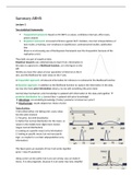
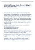
Empirical research uses collected data to learn from. Information in
this data is captured in a likelihood function, as in the figure on the
left.
Hereby you have the values of your parameter of interest on the X-
axis, and the likelihood for each value on the Y-axis.
In frequentist approach: all relevant information for inference is contained in the likelihood function
In Bayesian approach: in addition to the likelihood function to capture the information in the data,
we may also have prior information about µ (so we add something (the prior data)
Central idea/mechanism: prior knowledge is updated with information in the data and together
posterior distribution for µ (central idea + updated with prior knowledge)
Advantage: accumulating knowledge (‘today’s posterior is tomorrow’s prior’)
Disadvantage: results depend on choice of prior
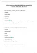
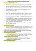
Type of priors:
1 Non-informative: not taking prior, every value
has the same chances
2. Flat prior, but with boundaries
3. Rather flat normal distribution for the mean, so
values in the middle have slight more chance
(vague normal distribution)
4. Looking at a specific mean (very informative)
5. looking at specific mean, but not necessarily
logic, so maybe for a certain subpopulation (very
informative)
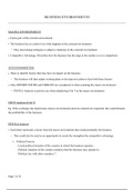
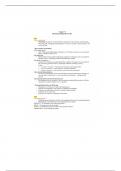
This figure gives an example of how it all works together
(prior + data posterior)
Using a prior can be useful, but is you are wrong, you can make it
worse. It is also pragmatic, because it is an easier way (you simplify)
,The posterior distribution of the parameter(s) of interest provides all desired estimates:
Posterior mean or mode: the mean or mode of the posterior distribution
Posterior SD: SD of posterior distribution (comparable to frequentist standard error) (how
wide the distribution is, tells you something about the uncertainty for that parameter)
Posterior 95% credible interval: providing the bounds of the part of the posterior in which
95% of the posterior mass is
(in the frequentist world they call it not a credible interval, but a confidence interval)
Hypothesis testing: looking at to which extent the data supports the hypothesis
p-value: probability of obtaining that result, or extremer
Your results (and conclusion) depend not on the observed data, but also the sampling plan. So the
same data can give different results, but this is not true in the Bayesian framework, because you
condition on the observed data
Bayes conditions on observed data, so it looks at the probability that hypothesis H j (not the same as
an H0 hypothesis) is supported by the data. Whereas frequentist testing conditions on H0, so with the
P-value (probability of observing same or more extreme data given that the null is true).
For the Bayesians it is important to get information on the probability that their hypothesis is true.
Therefore you can look at the PMP (posterior model probability); the probability of the hypothesis
after observing the data (and looking at the prior)
So the probability of a hypothesis being true depends on 2 criteria:
1. How sensible it is based on current knowledge (prior)
2. How well it fits new evidence (data)
Bayesian testing is comparative: hypotheses are
tested against one another, not in isolation
Posterior probabilities of hypotheses (PMP) are
also relative probabilities.
PMPs are an update of prior probabilities (for hypotheses) with the BF.
(the PMP’s are also comparative). You only compare the hypotheses that you stated as hypotheses of
interes
Both frameworks use probability theory, but (as if they use a different probability theory):
Frequentists: probability is relative frequency (more formal?)
Bayesians: probability is degree of belief (more intuitive?) (so the criticism is: is it still
objective)
This leads to debate (same word used for different things) and to differences in the correct
interpretation of statistical results. E.g., p-value vs PMP; also
Frequentist 95% confidence interval (CI): If we were tot repeat this experiment many times and
calculate a CI each time, 95% of the intervals will include the true parameter value (and 5% does not)
Bayesian 95% credible interval: There is 95% that the true value is in the credible interval
With Frequentist: it’s either yes or no, so reject or not, and with the Bayesian you can also compare.
, Paper By Hadlington:
It states: cyber security (of companies) is affected by the level of checking social media or the
internet for personal use during work time (cyberloafing).
With a multiple regression analysis, they investigated the effect of several predictors on the
outcome ISA (=information security awareness), i.e., age, gender, 5 personality traits, including FoMO
(Fear of Missing Out)
Key question: Does FoMo add to the prediction of ISA on top of all other predictors?
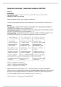
Linear regression:
In Scatterplot: X = independent variable (predictor), Y= dependent variable
(outcome)
The idea behind the linear regression model/estimation of the linear regression
model is the Least squares principle (distance between each observation and the
line represents the error in prediction (residuals), and the model/blue line
is drawn in a way that the sum of the squared residuals is as small as
possible
Error in prediction: difference between measured value and predicted
value
Multiple linear regression model:
In a multiple linear regression model, we still want to predict Y as in the ‘normal’ linear regression,
but here there are more variables.
An assumption here is that the residuals are approximately normally distributed
The observed outcome is a combination of the predicted outcome (model=additive linear model)
and the error in prediction
To estimate the model (estimating the b parameters and the residual variables), we check
assumptions, who have to be met.
With Model assumptions: All results are only reliable if assumptions by the model and approach
roughly hold:
Serious violations lead to incorrect results
Sometimes there are easy solutions (e.g. deleting a severe outlier; or
adding a quadratic term) and sometimes not (a few advanced solutions will also be
presented in this course)
Per model, know what the assumptions are and always check them carefully (see Grasple
lessons for theory and practice)
Basic assumption: MLR assumes interval/ratio variables (outcome and predictors)
Lecture 1
Two statistical frameworks:
Frequentist framework: Based on H0 (NHT), p-values, confidence intervals, effect sizes,
power analysis
Bayesian Framework: increased criticisms against NHT: mistakes, incorrect interpretations of
test results, p-hacking, over-emphasis on significance, underpowered studies, publication
bias
(there is an increasing use of the Bayesian framework over the Frequentist, because of the
replication crisis)
They both are part of empirical data.
Empirical research uses collected data to learn from. Information in
this data is captured in a likelihood function, as in the figure on the
left.
Hereby you have the values of your parameter of interest on the X-
axis, and the likelihood for each value on the Y-axis.
In frequentist approach: all relevant information for inference is contained in the likelihood function
In Bayesian approach: in addition to the likelihood function to capture the information in the data,
we may also have prior information about µ (so we add something (the prior data)
Central idea/mechanism: prior knowledge is updated with information in the data and together
posterior distribution for µ (central idea + updated with prior knowledge)
Advantage: accumulating knowledge (‘today’s posterior is tomorrow’s prior’)
Disadvantage: results depend on choice of prior
Type of priors:
1 Non-informative: not taking prior, every value
has the same chances
2. Flat prior, but with boundaries
3. Rather flat normal distribution for the mean, so
values in the middle have slight more chance
(vague normal distribution)
4. Looking at a specific mean (very informative)
5. looking at specific mean, but not necessarily
logic, so maybe for a certain subpopulation (very
informative)
This figure gives an example of how it all works together
(prior + data posterior)
Using a prior can be useful, but is you are wrong, you can make it
worse. It is also pragmatic, because it is an easier way (you simplify)
,The posterior distribution of the parameter(s) of interest provides all desired estimates:
Posterior mean or mode: the mean or mode of the posterior distribution
Posterior SD: SD of posterior distribution (comparable to frequentist standard error) (how
wide the distribution is, tells you something about the uncertainty for that parameter)
Posterior 95% credible interval: providing the bounds of the part of the posterior in which
95% of the posterior mass is
(in the frequentist world they call it not a credible interval, but a confidence interval)
Hypothesis testing: looking at to which extent the data supports the hypothesis
p-value: probability of obtaining that result, or extremer
Your results (and conclusion) depend not on the observed data, but also the sampling plan. So the
same data can give different results, but this is not true in the Bayesian framework, because you
condition on the observed data
Bayes conditions on observed data, so it looks at the probability that hypothesis H j (not the same as
an H0 hypothesis) is supported by the data. Whereas frequentist testing conditions on H0, so with the
P-value (probability of observing same or more extreme data given that the null is true).
For the Bayesians it is important to get information on the probability that their hypothesis is true.
Therefore you can look at the PMP (posterior model probability); the probability of the hypothesis
after observing the data (and looking at the prior)
So the probability of a hypothesis being true depends on 2 criteria:
1. How sensible it is based on current knowledge (prior)
2. How well it fits new evidence (data)
Bayesian testing is comparative: hypotheses are
tested against one another, not in isolation
Posterior probabilities of hypotheses (PMP) are
also relative probabilities.
PMPs are an update of prior probabilities (for hypotheses) with the BF.
(the PMP’s are also comparative). You only compare the hypotheses that you stated as hypotheses of
interes
Both frameworks use probability theory, but (as if they use a different probability theory):
Frequentists: probability is relative frequency (more formal?)
Bayesians: probability is degree of belief (more intuitive?) (so the criticism is: is it still
objective)
This leads to debate (same word used for different things) and to differences in the correct
interpretation of statistical results. E.g., p-value vs PMP; also
Frequentist 95% confidence interval (CI): If we were tot repeat this experiment many times and
calculate a CI each time, 95% of the intervals will include the true parameter value (and 5% does not)
Bayesian 95% credible interval: There is 95% that the true value is in the credible interval
With Frequentist: it’s either yes or no, so reject or not, and with the Bayesian you can also compare.
, Paper By Hadlington:
It states: cyber security (of companies) is affected by the level of checking social media or the
internet for personal use during work time (cyberloafing).
With a multiple regression analysis, they investigated the effect of several predictors on the
outcome ISA (=information security awareness), i.e., age, gender, 5 personality traits, including FoMO
(Fear of Missing Out)
Key question: Does FoMo add to the prediction of ISA on top of all other predictors?
Linear regression:
In Scatterplot: X = independent variable (predictor), Y= dependent variable
(outcome)
The idea behind the linear regression model/estimation of the linear regression
model is the Least squares principle (distance between each observation and the
line represents the error in prediction (residuals), and the model/blue line
is drawn in a way that the sum of the squared residuals is as small as
possible
Error in prediction: difference between measured value and predicted
value
Multiple linear regression model:
In a multiple linear regression model, we still want to predict Y as in the ‘normal’ linear regression,
but here there are more variables.
An assumption here is that the residuals are approximately normally distributed
The observed outcome is a combination of the predicted outcome (model=additive linear model)
and the error in prediction
To estimate the model (estimating the b parameters and the residual variables), we check
assumptions, who have to be met.
With Model assumptions: All results are only reliable if assumptions by the model and approach
roughly hold:
Serious violations lead to incorrect results
Sometimes there are easy solutions (e.g. deleting a severe outlier; or
adding a quadratic term) and sometimes not (a few advanced solutions will also be
presented in this course)
Per model, know what the assumptions are and always check them carefully (see Grasple
lessons for theory and practice)
Basic assumption: MLR assumes interval/ratio variables (outcome and predictors)