Linear Programming F a mke N o u we n s
Lecture 1
A linear program consists of:
- Objective function Z: function of decision variables (x1, .., xn) that we try to maximize or
minimize.
- Constraints:
• Functional: define the range of values for the decision variables
• Nonnegativity: the variable(s) are nonnegative. These need to be in the LP!
The constraints create a feasible region: a collection of solutions where all constraints are satisfied.
With an LP we assume:
- We only work with sums
- The decision variables are allowed to have any value that satisfies the constraints
- We assume that the value assigned to each parameter is a known constant.
- The optimal solution for an LP is always a corner-point of the feasible region.
There are two techniques for solving an LP:
- Simplex method (exterior-point method): goes along the border of the feasible region, one
corner-point at a time
- Interior-point method: goes through the middle of the feasible region (no corner-points).
This one is much slower than SM, but the number of iterations required increases much
more slowly than with the Simplex-method (so it’s better for large instances).
If we only have two decision variables, we can also use a graphical method, where we draw the
constraints in a graph and calculate the corner-points for optimality.
Lecture 2
An LP has a standard form:
- We maximize Z
- All decision variables are nonnegative (≥ 0)
- All functional constraints are of the form ≤
Real-world applications of LP’s:
- Maximum flow problem: constraints consist of the arc capacity constraints, the inflow =
outflow constraints, and the nonnegativity constraints. Side constraints can be:
• Minimum flow constraint (x1 should carry at least 3 units of flow: x1 3)
• Flow consumption constraint (node b keeps 2 units for itself: x2 = x3 + x4 + 2)
• Flow entering constraint (b is at most 5: x2 5).
- Linear regression problem: Minimize line y = ax + b by minimizing ∑ni=1 |(asi + b) − t i |. a
and b will be decision variables modeling the line and also use decision variables e1, …, en
measuring the vertical distance of point (s i,ti) from the line. So n+2 decision variables.
Minimize e1 + e2 + … + en
s.t. ei = |asi + b + ti| for each ei ≈ e1 as1 + b + t1 and e1 -(as1 + b + t1).
Once the core model has been stabilized for an LP, it is easy to add extra side constraints.
Lecture 3
When we have an LP, we have feasible and infeasible solutions. For the system to have a unique
solution we need one of these to be true:
, - Row-rank(C) = column-rank(C) = m
- All rows of C are linearly independent
- All columns of C are linearly independent
- C is invertible, so C-1 exists
If these conditions do not hold, then the system is either infeasible or
infinitely many solutions exists.
The simplex method only considers corner-point feasible solutions (CPF): a
solution where two or more constraints are equal. A solution is feasible if
and only if all the basic variables are ≥ 0.
The trick to solving an LP is to transfer the system into a higher dimension (= more decision
variables).
Dealing with constraints:
- ≤ : introduce a slack variable, that turns the constraint into =. It deals with the lack of the =
−constraint. If the slack variable is 0, it means the constraint is tight → the original variable
is sitting on the constraint boundary.
- = : introduce an artificial variable, that makes sure the Simplex method can start at the
origin.
- ≥ : introduce a surplus and an artificial variable. The surplus variable is the same as a slack
variable, but then deals with the excess.
If the LP is in standard form (Ax b), where A has m rows (constraints) and n columns (variables),
then the augmented form will consist of m equalities in m + n variables.
Lecture 4
Simplex method – method to solve an LP in standard form. Algorithm:
- We start with creating a basis: the
variables that are non-zero. In the
beginning these are the slack variables.
The size of the basis is the number of
functional constraints. Basic variables
never appear in the objective function!
- Determine the entering variable: the
variable that has the most potential to
improve Z and the leaving variable: the
row in the basis that has the highest
ratio: Z/coefficient of entering variable in
that row. Important, we only need to look at rows with strictly positive coefficients in the
pivot column!
- Use elementary row operations to create 0-1 pattern in column of entering variable and
repeat the process until there are no negative numbers in the top row anymore.
- The values for Z and the basic variables can be read off on the right-hand side.
Adjacent solutions – two solutions that have n – 1 constraint boundaries in common, ie. The two
sets of non-basic variables differ in exactly one variable.
There can be multiple optimal solutions, that can be explored by continuing to pivot after obtaining
an optimal CPF by choosing a non-basic variable with coefficient 0 in the top row as pivot column.
Some problems that can occur:
- No leaving basic variable → unbounded objective function
Lecture 1
A linear program consists of:
- Objective function Z: function of decision variables (x1, .., xn) that we try to maximize or
minimize.
- Constraints:
• Functional: define the range of values for the decision variables
• Nonnegativity: the variable(s) are nonnegative. These need to be in the LP!
The constraints create a feasible region: a collection of solutions where all constraints are satisfied.
With an LP we assume:
- We only work with sums
- The decision variables are allowed to have any value that satisfies the constraints
- We assume that the value assigned to each parameter is a known constant.
- The optimal solution for an LP is always a corner-point of the feasible region.
There are two techniques for solving an LP:
- Simplex method (exterior-point method): goes along the border of the feasible region, one
corner-point at a time
- Interior-point method: goes through the middle of the feasible region (no corner-points).
This one is much slower than SM, but the number of iterations required increases much
more slowly than with the Simplex-method (so it’s better for large instances).
If we only have two decision variables, we can also use a graphical method, where we draw the
constraints in a graph and calculate the corner-points for optimality.
Lecture 2
An LP has a standard form:
- We maximize Z
- All decision variables are nonnegative (≥ 0)
- All functional constraints are of the form ≤
Real-world applications of LP’s:
- Maximum flow problem: constraints consist of the arc capacity constraints, the inflow =
outflow constraints, and the nonnegativity constraints. Side constraints can be:
• Minimum flow constraint (x1 should carry at least 3 units of flow: x1 3)
• Flow consumption constraint (node b keeps 2 units for itself: x2 = x3 + x4 + 2)
• Flow entering constraint (b is at most 5: x2 5).
- Linear regression problem: Minimize line y = ax + b by minimizing ∑ni=1 |(asi + b) − t i |. a
and b will be decision variables modeling the line and also use decision variables e1, …, en
measuring the vertical distance of point (s i,ti) from the line. So n+2 decision variables.
Minimize e1 + e2 + … + en
s.t. ei = |asi + b + ti| for each ei ≈ e1 as1 + b + t1 and e1 -(as1 + b + t1).
Once the core model has been stabilized for an LP, it is easy to add extra side constraints.
Lecture 3
When we have an LP, we have feasible and infeasible solutions. For the system to have a unique
solution we need one of these to be true:
, - Row-rank(C) = column-rank(C) = m
- All rows of C are linearly independent
- All columns of C are linearly independent
- C is invertible, so C-1 exists
If these conditions do not hold, then the system is either infeasible or
infinitely many solutions exists.
The simplex method only considers corner-point feasible solutions (CPF): a
solution where two or more constraints are equal. A solution is feasible if
and only if all the basic variables are ≥ 0.
The trick to solving an LP is to transfer the system into a higher dimension (= more decision
variables).
Dealing with constraints:
- ≤ : introduce a slack variable, that turns the constraint into =. It deals with the lack of the =
−constraint. If the slack variable is 0, it means the constraint is tight → the original variable
is sitting on the constraint boundary.
- = : introduce an artificial variable, that makes sure the Simplex method can start at the
origin.
- ≥ : introduce a surplus and an artificial variable. The surplus variable is the same as a slack
variable, but then deals with the excess.
If the LP is in standard form (Ax b), where A has m rows (constraints) and n columns (variables),
then the augmented form will consist of m equalities in m + n variables.
Lecture 4
Simplex method – method to solve an LP in standard form. Algorithm:
- We start with creating a basis: the
variables that are non-zero. In the
beginning these are the slack variables.
The size of the basis is the number of
functional constraints. Basic variables
never appear in the objective function!
- Determine the entering variable: the
variable that has the most potential to
improve Z and the leaving variable: the
row in the basis that has the highest
ratio: Z/coefficient of entering variable in
that row. Important, we only need to look at rows with strictly positive coefficients in the
pivot column!
- Use elementary row operations to create 0-1 pattern in column of entering variable and
repeat the process until there are no negative numbers in the top row anymore.
- The values for Z and the basic variables can be read off on the right-hand side.
Adjacent solutions – two solutions that have n – 1 constraint boundaries in common, ie. The two
sets of non-basic variables differ in exactly one variable.
There can be multiple optimal solutions, that can be explored by continuing to pivot after obtaining
an optimal CPF by choosing a non-basic variable with coefficient 0 in the top row as pivot column.
Some problems that can occur:
- No leaving basic variable → unbounded objective function