Grasple week 1a – Refresh linear regression
1. Introduction
Simple linear regression – There’s only 1 independent variable in the model.
2. About correlation
In this lesson you will learn
- An easy to interpret standardised measure to express the strength of the linear
relationships between variables
We assume you know:
- How to assess the strength of the relationship based on a scatterplot
Pearson invented a standardized number to assess the strength of a linear relationship (between two
numerical variables), called the correlation coefficient
- An absolute value of 1 indicates maximum strength of a relation between two variables
- A value of 0 indicates no linear relation between the two variables
- Cohens d r n2
Weak 0.2 0.1 0.01
Medium 0.5 0.3 0.06
strong 0.8 0.5 0.14
- The correlation is a standardized measure, and multiple strengths of relationships can be
compared because of that.
- However, a low correlation or a correlation of 0 does not mean that there is no relation
between the two variables. The relationship can also be non-linear.
- Correlation doesn’t mean causation.
Summary - This lesson has taught you that:
- A correlation is a standardized measure of the strength of the linear relationship between
two variables.
- A correlation is scaled to always be between -1 and 1.
- A high positive correlation means that when one variable increases, the other one also
increases.
- A high negative correlation means that when one variable increases, the other one
decreases.
- A correlation of 0 means that when one variable increases, that has no linear influence on
the other variable
- A correlation of 0 does not mean that there is no relationship between the two variables, it
could be a non-linear relationship.
- A correlation does not say anything about the causal effects of the variables.
3. More on correlation and causality
The lesson will teach you:
- The difference between correlation and causation
- Why it is so important to keep the two apart
Pearson’s correlation and/or linear regression → interval/ratio niveau
,First: Draw scatterplot
Then: Pearson’s r allows you to compare correlations, because Pearson’s r is always between -1 and
1 → Standardized measure of strength of a linear relationship.
CORRELATION ≠ CAUSATION
• Voorwaarden causaliteit
1. Covariance (covariantie)
Er moet een relatie zijn tussen de oorzaak en het gevolg.
2. Temporal precedence (volgorde in tijd)
De oorzaak moet in de tijd voorafgaan aan het gevolg.
3. Internal validity (interne validiteit)
Alternatieve verklaringen voor de gevonden relatie moeten zijn uitgesloten = experimental
design.
Summary
- It is a common mistake to interpret a correlation between two variables as one variable
causing a change in the other.
- This difference is referred to as "correlation vs. causation".
- Be precise when reporting your conclusions based on a correlation. Otherwise people might
misquote your findings later on.
4. The linear regression model
This lesson will teach you:
- to think straight about linear regression.
- when to use linear regression.
- how to come up with a regression formula.
We assume you know:
- How to see if there is a relation between two variables from a scatterplot
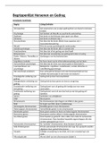
Different levels of variables
Categorische variabelen
- Voorbeeld:
• Variabele: Sekse
• Waarden: 1 = Man, 2 = Vrouw
- Voorbeeld:
• Variabele: Lievelingskleur
• Waarden: 1 = rood, 2 = blauw, …, 6 = paars
In beide gevallen vertegenwoordigen de getallen geen
hoeveelheden maar verschillende categorieën
Ordinaal meetniveau
- Wanneer de getallen aangeven dat de ene waarde meer/ groter/ hoger/ sterker is dan de
andere, maar niet met hoeveel:
- Voorbeeld:
• Variabele: Kledingmaat
• Waarden: 1 = XS, 2 = S, 3 = M, 4 = L, 5 = XL
,Interval meetniveau
- Wanneer de verschillen tussen getallen wél hetzelfde zijn, maar
• De waarde 0 (nul) is geen indicatie van de afwezigheid van de gemeten variabele
• Een waarde 2 of 3 keer zo groot geeft niet aan dat het 2 of 3 keer meer/ langer/ sterker
is.
- Voorbeeld:
• Variabele: IQ score
• Waarden: minimum = 60, maximum = 140
Ratio meetniveau
- Wanneer de verschillen tussen getallen hetzelfde zijn én de waarde 0 is een indicatie van de
afwezigheid van de gemeten variabele
- Voorbeeld:
• Variabele: Lichaamslengte van de participant
• Waarden: tussen 80-210 cm
Minimal measurement level for linear regression = INTERVAL/RATIO
First: Draw scatterplot
Then: Pearson’s r allows you to compare correlations, because Pearson’s r
is always between -1 and
1 → Standardized measure of strength of a linear relationship.
• Y = ax + b // ŷ = B0 + B1 * x
• First: calculate is the slope (B1) of the line (=vertical/horizontal).
• Second: Intercept = snijpunt y-as (B0)
➢ The intercept can be fairly meaningless and only serves
(mathematically) to support a correct prediction →
interpretation of this can be non-sensical.
• Ŷ is predicted y-score (≠ observed)
Summary - In this lesson you have learned that:
- Linear regression is an analysis in which you attempt to summarise a bunch of data points by
drawing a straight line through them
- Linear regression requires variables at interval/ratio level
- Linear regression should only be performed on linear relations
- The regression equation can be written as: ŷ = B0 + B1 * x
- B0 refers to the intercept, the point where the line crosses the y-axis and is interpreted as: if
X is 0, Y is ...
- B1 refers to the slope of the line and is interpreted as: if X increases by 1 unit, Y
increases/decreases by ....units.
5. Estimating the regression line
In this lesson you will learn:
- What a regression line is and how it is calculated
- What the least squares method is
This brings us to the question: where exactly to draw this line? → least squares method
, The predicted y values are the same, but the observed y values can be
different.
- The predicted value is the corresponding y-value on the
regression line (in the graph called ‘expected value’), whilst the
observed scores can differ
- The difference between them two (Y - Ŷ) = error or residual
- Ŷ = predicted y-score
- Y = observed y-score
The sum of all errors then is always zero, therefore we use:
- Least squares method.
When we square the errors, they will always be positive and they
do not cancel each other. This way we can look for the line that will result in the smallest
possible sum of squared errors.
• Om te voorkomen dat de geobserveerde scores onder de regression line en de scores
boven de lijn elkaar uitmiddelen en samen tot een sum van 0 komen.
- De formule voor smallest sum of sq. errors; So the slope equals the
correlation coefficient (pearson's r) times the standard deviation of y
divided by the standard deviation of x.
• You don’t need to know the formula, just be sure
you can read the output.
- Intercept lees je af in de ‘’COEFFICIENTS’’-tabel = constant
- Slope idem, is onderste waarde
Summary - In this lesson you learned that:
- A regression line never fits all the data points perfectly. There will always be a residual error.
- This residual error is the difference between observed scores y and predicted scores y hat →
(Y - Ŷ)
- The estimated regression model is based on reducing the sum of the squared errors,
to a minimum.
- This least squares principle provides formula for how to compute the slope and intercept of
the best fitting linear regression line. SPSS (or other statistical software) provides these
estimates for you.
- Its used to estimate the parameters of the linear regression model (to find the linear
regression which fits the data best)
6. R-squared
In this lesson you will learn:
- Why you look at an R-squared
- How to correctly interpret an R-squared
We assume that you already know:
- What a proportion is
- Conceptually what a linear regression is
Predicting a rating based on the budget is an example of a simple linear regression.
- Dependent/outcome = rating
- Independent/predictor = budget
1. Introduction
Simple linear regression – There’s only 1 independent variable in the model.
2. About correlation
In this lesson you will learn
- An easy to interpret standardised measure to express the strength of the linear
relationships between variables
We assume you know:
- How to assess the strength of the relationship based on a scatterplot
Pearson invented a standardized number to assess the strength of a linear relationship (between two
numerical variables), called the correlation coefficient
- An absolute value of 1 indicates maximum strength of a relation between two variables
- A value of 0 indicates no linear relation between the two variables
- Cohens d r n2
Weak 0.2 0.1 0.01
Medium 0.5 0.3 0.06
strong 0.8 0.5 0.14
- The correlation is a standardized measure, and multiple strengths of relationships can be
compared because of that.
- However, a low correlation or a correlation of 0 does not mean that there is no relation
between the two variables. The relationship can also be non-linear.
- Correlation doesn’t mean causation.
Summary - This lesson has taught you that:
- A correlation is a standardized measure of the strength of the linear relationship between
two variables.
- A correlation is scaled to always be between -1 and 1.
- A high positive correlation means that when one variable increases, the other one also
increases.
- A high negative correlation means that when one variable increases, the other one
decreases.
- A correlation of 0 means that when one variable increases, that has no linear influence on
the other variable
- A correlation of 0 does not mean that there is no relationship between the two variables, it
could be a non-linear relationship.
- A correlation does not say anything about the causal effects of the variables.
3. More on correlation and causality
The lesson will teach you:
- The difference between correlation and causation
- Why it is so important to keep the two apart
Pearson’s correlation and/or linear regression → interval/ratio niveau
,First: Draw scatterplot
Then: Pearson’s r allows you to compare correlations, because Pearson’s r is always between -1 and
1 → Standardized measure of strength of a linear relationship.
CORRELATION ≠ CAUSATION
• Voorwaarden causaliteit
1. Covariance (covariantie)
Er moet een relatie zijn tussen de oorzaak en het gevolg.
2. Temporal precedence (volgorde in tijd)
De oorzaak moet in de tijd voorafgaan aan het gevolg.
3. Internal validity (interne validiteit)
Alternatieve verklaringen voor de gevonden relatie moeten zijn uitgesloten = experimental
design.
Summary
- It is a common mistake to interpret a correlation between two variables as one variable
causing a change in the other.
- This difference is referred to as "correlation vs. causation".
- Be precise when reporting your conclusions based on a correlation. Otherwise people might
misquote your findings later on.
4. The linear regression model
This lesson will teach you:
- to think straight about linear regression.
- when to use linear regression.
- how to come up with a regression formula.
We assume you know:
- How to see if there is a relation between two variables from a scatterplot
Different levels of variables
Categorische variabelen
- Voorbeeld:
• Variabele: Sekse
• Waarden: 1 = Man, 2 = Vrouw
- Voorbeeld:
• Variabele: Lievelingskleur
• Waarden: 1 = rood, 2 = blauw, …, 6 = paars
In beide gevallen vertegenwoordigen de getallen geen
hoeveelheden maar verschillende categorieën
Ordinaal meetniveau
- Wanneer de getallen aangeven dat de ene waarde meer/ groter/ hoger/ sterker is dan de
andere, maar niet met hoeveel:
- Voorbeeld:
• Variabele: Kledingmaat
• Waarden: 1 = XS, 2 = S, 3 = M, 4 = L, 5 = XL
,Interval meetniveau
- Wanneer de verschillen tussen getallen wél hetzelfde zijn, maar
• De waarde 0 (nul) is geen indicatie van de afwezigheid van de gemeten variabele
• Een waarde 2 of 3 keer zo groot geeft niet aan dat het 2 of 3 keer meer/ langer/ sterker
is.
- Voorbeeld:
• Variabele: IQ score
• Waarden: minimum = 60, maximum = 140
Ratio meetniveau
- Wanneer de verschillen tussen getallen hetzelfde zijn én de waarde 0 is een indicatie van de
afwezigheid van de gemeten variabele
- Voorbeeld:
• Variabele: Lichaamslengte van de participant
• Waarden: tussen 80-210 cm
Minimal measurement level for linear regression = INTERVAL/RATIO
First: Draw scatterplot
Then: Pearson’s r allows you to compare correlations, because Pearson’s r
is always between -1 and
1 → Standardized measure of strength of a linear relationship.
• Y = ax + b // ŷ = B0 + B1 * x
• First: calculate is the slope (B1) of the line (=vertical/horizontal).
• Second: Intercept = snijpunt y-as (B0)
➢ The intercept can be fairly meaningless and only serves
(mathematically) to support a correct prediction →
interpretation of this can be non-sensical.
• Ŷ is predicted y-score (≠ observed)
Summary - In this lesson you have learned that:
- Linear regression is an analysis in which you attempt to summarise a bunch of data points by
drawing a straight line through them
- Linear regression requires variables at interval/ratio level
- Linear regression should only be performed on linear relations
- The regression equation can be written as: ŷ = B0 + B1 * x
- B0 refers to the intercept, the point where the line crosses the y-axis and is interpreted as: if
X is 0, Y is ...
- B1 refers to the slope of the line and is interpreted as: if X increases by 1 unit, Y
increases/decreases by ....units.
5. Estimating the regression line
In this lesson you will learn:
- What a regression line is and how it is calculated
- What the least squares method is
This brings us to the question: where exactly to draw this line? → least squares method
, The predicted y values are the same, but the observed y values can be
different.
- The predicted value is the corresponding y-value on the
regression line (in the graph called ‘expected value’), whilst the
observed scores can differ
- The difference between them two (Y - Ŷ) = error or residual
- Ŷ = predicted y-score
- Y = observed y-score
The sum of all errors then is always zero, therefore we use:
- Least squares method.
When we square the errors, they will always be positive and they
do not cancel each other. This way we can look for the line that will result in the smallest
possible sum of squared errors.
• Om te voorkomen dat de geobserveerde scores onder de regression line en de scores
boven de lijn elkaar uitmiddelen en samen tot een sum van 0 komen.
- De formule voor smallest sum of sq. errors; So the slope equals the
correlation coefficient (pearson's r) times the standard deviation of y
divided by the standard deviation of x.
• You don’t need to know the formula, just be sure
you can read the output.
- Intercept lees je af in de ‘’COEFFICIENTS’’-tabel = constant
- Slope idem, is onderste waarde
Summary - In this lesson you learned that:
- A regression line never fits all the data points perfectly. There will always be a residual error.
- This residual error is the difference between observed scores y and predicted scores y hat →
(Y - Ŷ)
- The estimated regression model is based on reducing the sum of the squared errors,
to a minimum.
- This least squares principle provides formula for how to compute the slope and intercept of
the best fitting linear regression line. SPSS (or other statistical software) provides these
estimates for you.
- Its used to estimate the parameters of the linear regression model (to find the linear
regression which fits the data best)
6. R-squared
In this lesson you will learn:
- Why you look at an R-squared
- How to correctly interpret an R-squared
We assume that you already know:
- What a proportion is
- Conceptually what a linear regression is
Predicting a rating based on the budget is an example of a simple linear regression.
- Dependent/outcome = rating
- Independent/predictor = budget