Chapter 15
The Hamiltonian method
Copyright 2008 by David Morin, (Draft Version 2, October 2008)
This chapter is to be read in conjunction with Introduction to Classical Mechanics, With Problems
and Solutions ° c 2007, by David Morin, Cambridge University Press.
The text in this version is the same as in Version 1, but some new problems and exercises have
been added.
More information on the book can be found at:
http://www.people.fas.harvard.edu/˜djmorin/book.html
At present, we have at our disposal two basic ways of solving mechanics problems. In
Chapter 3 we discussed the familiar method involving Newton’s laws, in particular
the second law, F = ma. And in Chapter 6 we learned about the Lagrangian
method. These two strategies always yield the same results for a given problem, of
course, but they are based on vastly different principles. Depending on the specifics
of the problem at hand, one method might lead to a simpler solution than the other.
In this chapter, we’ll learn about a third way of solving problems, the Hamil-
tonian method. This method is quite similar to the Lagrangian method, so it’s
debateable as to whether it should actually count as a third one. Like the La-
grangian method, it contains the principle of stationary action as an ingredient.
But it also contains many additional features that are extremely useful in other
branches of physics, in particular statistical mechanics and quantum mechanics.
Although the Hamiltonian method generally has no advantage over (and in fact is
invariably much more cumbersome than) the Lagrangian method when it comes to
standard mechanics problems involving a small number of particles, its superiority
becomes evident when dealing with systems at the opposite ends of the spectrum
compared with “a small number of particles,” namely systems with an intractably
large number of particles (as in a statistical-mechanics system involving a gas), or
systems with no particles at all (as in quantum mechanics, where everything is a
wave).
We won’t be getting into these topics here, so you’ll have to take it on faith
how useful the Hamiltonian formalism is. Furthermore, since much of this book is
based on problem solving, this chapter probably won’t be the most rewarding one,
because there is rarely any benefit from using a Hamiltonian instead of a Lagrangian
to solve a standard mechanics problem. Indeed, many of the examples and problems
in this chapter might seem a bit silly, considering that they can be solved much more
quickly using the Lagrangian method. But rest assured, this silliness has a purpose;
the techniques you learn here will be very valuable in your future physics studies.
The outline of this chapter is as follows. In Section 15.1 we’ll look at the sim-
XV-1
,XV-2 CHAPTER 15. THE HAMILTONIAN METHOD
ilarities between the Hamiltonian and the energy, and then in Section 15.2 we’ll
rigorously define the Hamiltonian and derive Hamilton’s equations, which are the
equations that take the place of Newton’s laws and the Euler-Lagrange equations.
In Section 15.3 we’ll discuss the Legendre transform, which is what connects the
Hamiltonian to the Lagrangian. In Section 15.4 we’ll give three more derivations of
Hamilton’s equations, just for the fun of it. Finally, in Section 15.5 we’ll introduce
the concept of phase space and then derive Liouville’s theorem, which has countless
applications in statistical mechanics, chaos, and other fields.
15.1 Energy
In Eq. (6.52) in Chapter 6 we defined the quantity,
ÃN !
X ∂L
E≡ q̇i − L, (15.1)
i=1
∂ q̇i
which under many circumstances is the energy of the system, as we will see below.
We then showed in Claim 6.3 that dE/dt = −∂L/∂t. This implies that if ∂L/∂t = 0
(that is, if t doesn’t explicitly appear in L), then E is constant in time. In the
present chapter, we will examine many other properties of this quantity E, or more
precisely, the quantity H (the Hamiltonian) that arises when E is rewritten in a
certain way explained in Section 15.2.1.
But before getting into a detailed discussion of the actual Hamiltonian, let’s first
look at the relation between E and the energy of the system. We chose the letter
E in Eq. (6.52/15.1) because the quantity on the right-hand side often turns out to
be the total energy of the system. For example, consider a particle undergoing 1-D
motion under the influence of a potential V (x), where x is a standard Cartesian
coordinate. Then L ≡ T − V = mẋ2 /2 − V (x), which yields
∂L
E≡ ẋ − L = (mẋ)ẋ − L = 2T − (T − V ) = T + V, (15.2)
∂ ẋ
which is simply the total energy. By performing the analogous calculation, it like-
wise follows that E is the total energy in the case of Cartesian coordinates in N
dimensions:
µ 
1 1
L = mẋ21 + · · · + mẋ2N − V (x1 , . . . , xN )
2 2
³ ´
=⇒ E = (mẋ1 )ẋ1 + · · · + (mẋN )ẋN − L
= 2T − (T − V )
= T + V. (15.3)
In view of this, a reasonable question to ask is: Does E always turn out to be the
total energy, no matter what coordinates are used to describe the system? Alas,
the answer is no. However, when the coordinates satisfy a certain condition, E is
indeed the total energy. Let’s see what this condition is.
Consider a slight modification to the above 1-D setup. We’ll change variables
from the nice Cartesian coordinate x to another coordinate q defined by, say, x(q) =
Kq 5 , or equivalently q(x) = (x/K)1/5 . Since ẋ = 5Kq 4 q̇, we can rewrite the
Lagrangian L(x, ẋ) = mẋ2 /2 − V (x) in terms of q and q̇ as
µ 
25K 2 mq 8 ¡ ¢
L(q, q̇) = q̇ 2 − V x(q) ≡ F (q)q̇ 2 − Vu (q), (15.4)
2
,15.1. ENERGY XV-3
where F (q) ≡ 25K 2 mq 8 /2 (so the kinetic energy is T = F (q)q̇ 2 ). The quantity E
is then
∂L ¡ ¢
E≡ q̇ − L = 2F (q)q̇ q̇ − L = 2T − (T − V ) = T + V, (15.5)
∂ q̇
which again is the total energy. So apparently it is possible for (at least some)
non-Cartesian coordinates to yield an E equaling the total energy.
We can easily demonstrate that in 1-D, E equals the total energy if the new
coordinate q is related to the old Cartesian coordinate x by any general functional
dependence of the form, x = x(q). The reason is that since ẋ = (dx/dq)q̇ by the
chain rule, the kinetic energy always takes the form of q̇ 2 times some function of q.
That is, T = F (q)q̇ 2 , where F (q) happens to be (m/2)(dx/dq)2 . This function F (q)
just goes along for the ride in the calculation of E, so the result of T + V arises in
exactly the same way as in Eq. (15.5).
What if instead of the simple relation x = x(q) (or equivalently q = q(x)) we
also have time dependence? That is, x = x(q, t) (or equivalently q = q(x, t))? The
task of Problem 15.1 is to show that L(q, q̇, t) yields an E that takes the form,
õ ¶ µ ¶ µ ¶2 !
∂x ∂x ∂x
E =T +V −m q̇ + , (15.6)
∂q ∂t ∂t
which is not the total energy, T + V , due to the ∂x(q, t)/∂t 6= 0 assumption. So a
necessary condition for E to be the total energy is that there is no time dependence
when the Cartesian coordinates are written in terms of the new coordinates (or vice
versa).
Likewise, you can show that if there is q̇ dependence, so that x = x(q, q̇), the
resulting E turns out to be a very large mess that doesn’t equal T + V . However,
this point is moot, because as we did in Chapter 6, we will assume that the trans-
formation between two sets of coordinates never involves the time derivatives of the
coordinates.
So far we’ve dealt with only one variable. What about two? In terms of Carte-
sian coordinates, the Lagrangian is L = (m/2)(ẋ21 + ẋ22 ) − V (x1 , x2 ). If these co-
ordinates are related to new ones (call them q1 and q2 ) by x1 = x1 (q1 , q2 ) and
x2 = x2 (q1 , q2 ), then we have x˙1 = (∂x1 /∂q1 )q̇1 + (∂x1 /∂q2 )q̇2 , and similarly for ẋ2 .
Therefore, when written in terms of the q’s, the kinetic energy takes the form,
m
T = (Aq̇12 + B q̇1 q̇2 + C q̇22 ), (15.7)
2
where A, B, and C are various functions of the q’s (but not the q̇’s), the exact forms
of which won’t be necessary here. So in terms of the new coordinates, we have
∂L ∂L
E = q̇1 + q̇2 − L
∂ q̇1 ∂ q̇2
³ ´ ³ ´
= m Aq̇1 + (B/2)q̇2 q̇1 + m (B/2)q̇1 + C q̇2 q̇2 − L
¡ ¢
= m Aq̇12 + B q̇1 q̇2 + C q̇22 − L
= 2T − (T − V )
= T + V, (15.8)
which is the total energy. This reasoning quickly generalizes to N coordinates, qi .
The kinetic energy has only two types of terms: ones that involve q̇i2 and ones that
, XV-4 CHAPTER 15. THE HAMILTONIAN METHOD
involve q̇i q̇j . These both pick upP
a factor of 2 (as either a 2 or a 1 + 1, as we just
saw in the 2-D case) in the sum (∂L/∂ q̇i )q̇i , thereby yielding 2T .
As in the 1-D case, time dependence in the relation between the Cartesian
coordinates and the new coordinates will cause E to not be the total energy, as
we saw in Eq. (15.6) for the 1-D case. And again, q̇i dependence will also have
this effect, but we are excluding such dependence. We can sum up all of the above
results by saying:
Theorem 15.1 A necessary and sufficient condition for the quantity E to be the
total energy of a system whose Lagrangian is written in terms of a set of coordinates
qi is that these qi are related to a Cartesian set of coordinates xi via expressions of
the form,
x1 = x1 (q1 , q2 , . . .),
..
.
xN = xN (q1 , q2 , . . .). (15.9)
That is, there is no t or q̇i dependence.
In theory, these relations can be inverted to write the qi as functions of the xi .
Remark: It is quite permissible for the number of qi ’s to be smaller than the number of
Cartesian xi ’s (N in Eq. (15.9)). Such is the case when there are constraints in the system.
For example, if a particle is constrained to move on a plane inclined at a given angle θ,
then (assuming that the origin is chosen to be on the plane) the Cartesian coordinates
(x, y) are related to the distance along the plane, r, by x = r cos θ and y = r sin θ. Because
θ is given, we therefore have only one qi , namely q1 ≡ r.1 The point is that
P 2even if there
are fewer than N qi ’s, the kinetic energy still takes the form of (m/2) ẋi in terms of
Cartesian coordinates, and so it still takes the form (in the case of two qi ’s) given in Eq.
(15.7) once the constraints have been invoked and the number of coordinates reduced (so
that the Lagrangian can be expressed in terms of independent coordinates, which is a
requirement in the Lagrangian formalism). So E still ends up being the energy (assuming
there is no t or q̇i dependence in the transformations).
Note that if the system is describable in terms of Cartesian coordinates (which means
that either there are no constraints, or the constraints are sufficiently simple), and if we
do in fact use these coordinates, then as we showed in Eq. (15.3), E is always the energy.
♣
y
Example 1 (Particle in a plane): A particle of mass m moves in a horizontal
x plane. It is connected to the origin by a spring with spring constant k and relaxed
length zero (so the potential energy is kr2 /2 = k(x2 + y 2 )/2), as shown in Fig. 15.1.
Find L and E in terms of Cartesian coordinates, and then also in terms of polar
coordinates. Verify that in both cases, E is the energy and it is conserved.
Solution: In Cartesian coordinates, we have
Figure 15.1
m 2 k
L=T −V = (ẋ + ẏ 2 ) − (x2 + y 2 ), (15.10)
2 2
1 A more trivial example is a particle constrained to move in the x-y plane. In this case, the
Cartesian coordinates (x, y, z) are related to the “new” coordinates (q1 , q2 ) in the plane (which we
will take to be equal to x and y) by the relations: x = q1 , y = q2 , and z = 0.
The Hamiltonian method
Copyright 2008 by David Morin, (Draft Version 2, October 2008)
This chapter is to be read in conjunction with Introduction to Classical Mechanics, With Problems
and Solutions ° c 2007, by David Morin, Cambridge University Press.
The text in this version is the same as in Version 1, but some new problems and exercises have
been added.
More information on the book can be found at:
http://www.people.fas.harvard.edu/˜djmorin/book.html
At present, we have at our disposal two basic ways of solving mechanics problems. In
Chapter 3 we discussed the familiar method involving Newton’s laws, in particular
the second law, F = ma. And in Chapter 6 we learned about the Lagrangian
method. These two strategies always yield the same results for a given problem, of
course, but they are based on vastly different principles. Depending on the specifics
of the problem at hand, one method might lead to a simpler solution than the other.
In this chapter, we’ll learn about a third way of solving problems, the Hamil-
tonian method. This method is quite similar to the Lagrangian method, so it’s
debateable as to whether it should actually count as a third one. Like the La-
grangian method, it contains the principle of stationary action as an ingredient.
But it also contains many additional features that are extremely useful in other
branches of physics, in particular statistical mechanics and quantum mechanics.
Although the Hamiltonian method generally has no advantage over (and in fact is
invariably much more cumbersome than) the Lagrangian method when it comes to
standard mechanics problems involving a small number of particles, its superiority
becomes evident when dealing with systems at the opposite ends of the spectrum
compared with “a small number of particles,” namely systems with an intractably
large number of particles (as in a statistical-mechanics system involving a gas), or
systems with no particles at all (as in quantum mechanics, where everything is a
wave).
We won’t be getting into these topics here, so you’ll have to take it on faith
how useful the Hamiltonian formalism is. Furthermore, since much of this book is
based on problem solving, this chapter probably won’t be the most rewarding one,
because there is rarely any benefit from using a Hamiltonian instead of a Lagrangian
to solve a standard mechanics problem. Indeed, many of the examples and problems
in this chapter might seem a bit silly, considering that they can be solved much more
quickly using the Lagrangian method. But rest assured, this silliness has a purpose;
the techniques you learn here will be very valuable in your future physics studies.
The outline of this chapter is as follows. In Section 15.1 we’ll look at the sim-
XV-1
,XV-2 CHAPTER 15. THE HAMILTONIAN METHOD
ilarities between the Hamiltonian and the energy, and then in Section 15.2 we’ll
rigorously define the Hamiltonian and derive Hamilton’s equations, which are the
equations that take the place of Newton’s laws and the Euler-Lagrange equations.
In Section 15.3 we’ll discuss the Legendre transform, which is what connects the
Hamiltonian to the Lagrangian. In Section 15.4 we’ll give three more derivations of
Hamilton’s equations, just for the fun of it. Finally, in Section 15.5 we’ll introduce
the concept of phase space and then derive Liouville’s theorem, which has countless
applications in statistical mechanics, chaos, and other fields.
15.1 Energy
In Eq. (6.52) in Chapter 6 we defined the quantity,
ÃN !
X ∂L
E≡ q̇i − L, (15.1)
i=1
∂ q̇i
which under many circumstances is the energy of the system, as we will see below.
We then showed in Claim 6.3 that dE/dt = −∂L/∂t. This implies that if ∂L/∂t = 0
(that is, if t doesn’t explicitly appear in L), then E is constant in time. In the
present chapter, we will examine many other properties of this quantity E, or more
precisely, the quantity H (the Hamiltonian) that arises when E is rewritten in a
certain way explained in Section 15.2.1.
But before getting into a detailed discussion of the actual Hamiltonian, let’s first
look at the relation between E and the energy of the system. We chose the letter
E in Eq. (6.52/15.1) because the quantity on the right-hand side often turns out to
be the total energy of the system. For example, consider a particle undergoing 1-D
motion under the influence of a potential V (x), where x is a standard Cartesian
coordinate. Then L ≡ T − V = mẋ2 /2 − V (x), which yields
∂L
E≡ ẋ − L = (mẋ)ẋ − L = 2T − (T − V ) = T + V, (15.2)
∂ ẋ
which is simply the total energy. By performing the analogous calculation, it like-
wise follows that E is the total energy in the case of Cartesian coordinates in N
dimensions:
µ 
1 1
L = mẋ21 + · · · + mẋ2N − V (x1 , . . . , xN )
2 2
³ ´
=⇒ E = (mẋ1 )ẋ1 + · · · + (mẋN )ẋN − L
= 2T − (T − V )
= T + V. (15.3)
In view of this, a reasonable question to ask is: Does E always turn out to be the
total energy, no matter what coordinates are used to describe the system? Alas,
the answer is no. However, when the coordinates satisfy a certain condition, E is
indeed the total energy. Let’s see what this condition is.
Consider a slight modification to the above 1-D setup. We’ll change variables
from the nice Cartesian coordinate x to another coordinate q defined by, say, x(q) =
Kq 5 , or equivalently q(x) = (x/K)1/5 . Since ẋ = 5Kq 4 q̇, we can rewrite the
Lagrangian L(x, ẋ) = mẋ2 /2 − V (x) in terms of q and q̇ as
µ 
25K 2 mq 8 ¡ ¢
L(q, q̇) = q̇ 2 − V x(q) ≡ F (q)q̇ 2 − Vu (q), (15.4)
2
,15.1. ENERGY XV-3
where F (q) ≡ 25K 2 mq 8 /2 (so the kinetic energy is T = F (q)q̇ 2 ). The quantity E
is then
∂L ¡ ¢
E≡ q̇ − L = 2F (q)q̇ q̇ − L = 2T − (T − V ) = T + V, (15.5)
∂ q̇
which again is the total energy. So apparently it is possible for (at least some)
non-Cartesian coordinates to yield an E equaling the total energy.
We can easily demonstrate that in 1-D, E equals the total energy if the new
coordinate q is related to the old Cartesian coordinate x by any general functional
dependence of the form, x = x(q). The reason is that since ẋ = (dx/dq)q̇ by the
chain rule, the kinetic energy always takes the form of q̇ 2 times some function of q.
That is, T = F (q)q̇ 2 , where F (q) happens to be (m/2)(dx/dq)2 . This function F (q)
just goes along for the ride in the calculation of E, so the result of T + V arises in
exactly the same way as in Eq. (15.5).
What if instead of the simple relation x = x(q) (or equivalently q = q(x)) we
also have time dependence? That is, x = x(q, t) (or equivalently q = q(x, t))? The
task of Problem 15.1 is to show that L(q, q̇, t) yields an E that takes the form,
õ ¶ µ ¶ µ ¶2 !
∂x ∂x ∂x
E =T +V −m q̇ + , (15.6)
∂q ∂t ∂t
which is not the total energy, T + V , due to the ∂x(q, t)/∂t 6= 0 assumption. So a
necessary condition for E to be the total energy is that there is no time dependence
when the Cartesian coordinates are written in terms of the new coordinates (or vice
versa).
Likewise, you can show that if there is q̇ dependence, so that x = x(q, q̇), the
resulting E turns out to be a very large mess that doesn’t equal T + V . However,
this point is moot, because as we did in Chapter 6, we will assume that the trans-
formation between two sets of coordinates never involves the time derivatives of the
coordinates.
So far we’ve dealt with only one variable. What about two? In terms of Carte-
sian coordinates, the Lagrangian is L = (m/2)(ẋ21 + ẋ22 ) − V (x1 , x2 ). If these co-
ordinates are related to new ones (call them q1 and q2 ) by x1 = x1 (q1 , q2 ) and
x2 = x2 (q1 , q2 ), then we have x˙1 = (∂x1 /∂q1 )q̇1 + (∂x1 /∂q2 )q̇2 , and similarly for ẋ2 .
Therefore, when written in terms of the q’s, the kinetic energy takes the form,
m
T = (Aq̇12 + B q̇1 q̇2 + C q̇22 ), (15.7)
2
where A, B, and C are various functions of the q’s (but not the q̇’s), the exact forms
of which won’t be necessary here. So in terms of the new coordinates, we have
∂L ∂L
E = q̇1 + q̇2 − L
∂ q̇1 ∂ q̇2
³ ´ ³ ´
= m Aq̇1 + (B/2)q̇2 q̇1 + m (B/2)q̇1 + C q̇2 q̇2 − L
¡ ¢
= m Aq̇12 + B q̇1 q̇2 + C q̇22 − L
= 2T − (T − V )
= T + V, (15.8)
which is the total energy. This reasoning quickly generalizes to N coordinates, qi .
The kinetic energy has only two types of terms: ones that involve q̇i2 and ones that
, XV-4 CHAPTER 15. THE HAMILTONIAN METHOD
involve q̇i q̇j . These both pick upP
a factor of 2 (as either a 2 or a 1 + 1, as we just
saw in the 2-D case) in the sum (∂L/∂ q̇i )q̇i , thereby yielding 2T .
As in the 1-D case, time dependence in the relation between the Cartesian
coordinates and the new coordinates will cause E to not be the total energy, as
we saw in Eq. (15.6) for the 1-D case. And again, q̇i dependence will also have
this effect, but we are excluding such dependence. We can sum up all of the above
results by saying:
Theorem 15.1 A necessary and sufficient condition for the quantity E to be the
total energy of a system whose Lagrangian is written in terms of a set of coordinates
qi is that these qi are related to a Cartesian set of coordinates xi via expressions of
the form,
x1 = x1 (q1 , q2 , . . .),
..
.
xN = xN (q1 , q2 , . . .). (15.9)
That is, there is no t or q̇i dependence.
In theory, these relations can be inverted to write the qi as functions of the xi .
Remark: It is quite permissible for the number of qi ’s to be smaller than the number of
Cartesian xi ’s (N in Eq. (15.9)). Such is the case when there are constraints in the system.
For example, if a particle is constrained to move on a plane inclined at a given angle θ,
then (assuming that the origin is chosen to be on the plane) the Cartesian coordinates
(x, y) are related to the distance along the plane, r, by x = r cos θ and y = r sin θ. Because
θ is given, we therefore have only one qi , namely q1 ≡ r.1 The point is that
P 2even if there
are fewer than N qi ’s, the kinetic energy still takes the form of (m/2) ẋi in terms of
Cartesian coordinates, and so it still takes the form (in the case of two qi ’s) given in Eq.
(15.7) once the constraints have been invoked and the number of coordinates reduced (so
that the Lagrangian can be expressed in terms of independent coordinates, which is a
requirement in the Lagrangian formalism). So E still ends up being the energy (assuming
there is no t or q̇i dependence in the transformations).
Note that if the system is describable in terms of Cartesian coordinates (which means
that either there are no constraints, or the constraints are sufficiently simple), and if we
do in fact use these coordinates, then as we showed in Eq. (15.3), E is always the energy.
♣
y
Example 1 (Particle in a plane): A particle of mass m moves in a horizontal
x plane. It is connected to the origin by a spring with spring constant k and relaxed
length zero (so the potential energy is kr2 /2 = k(x2 + y 2 )/2), as shown in Fig. 15.1.
Find L and E in terms of Cartesian coordinates, and then also in terms of polar
coordinates. Verify that in both cases, E is the energy and it is conserved.
Solution: In Cartesian coordinates, we have
Figure 15.1
m 2 k
L=T −V = (ẋ + ẏ 2 ) − (x2 + y 2 ), (15.10)
2 2
1 A more trivial example is a particle constrained to move in the x-y plane. In this case, the
Cartesian coordinates (x, y, z) are related to the “new” coordinates (q1 , q2 ) in the plane (which we
will take to be equal to x and y) by the relations: x = q1 , y = q2 , and z = 0.