SOLUTION MANUAL
Modeling and Analysis of Dynamic Systems 3/E Ramin Esfandiari 1
Review Problems
=
1 Evaluate the function f ( x, y ) 23 e − x /2 cos( y − 1) for x =
−0.23, y =
2.7
(a) Using the subs command.
(b) By conversion into a MATLAB function.
Solution
(a)
>> f = sym('2*exp(-x/2)*cos(y-1)/3');
>> x = -0.23; y = 2.7;
>> double(subs(f))
ans =
-0.0964
(b)
>> F = matlabFunction(f);
>> F(-0.23,2.7)
ans =
-0.0964
2 Evaluate the function g ( x, y ) =sin(2 x + 1) tan( y − 12 ) for x = 0.45, y = −1.17
(a) Using the subs command.
(b) By conversion into a MATLAB function.
Solution
(a)
>> g = sym('sin(2*x+1)*tan(y-1/2)');
>> x = 0.45; y = -1.17;
>> double(subs(g))
ans =
9.5076
(b)
>> G = matlabFunction(g);
>> G(0.45,-1.17)
ans =
9.5076
xy + 1
3 Evaluate the vector function v( x, y ) = = =
for x 1.54, y 2.28
x − 2 y
(a) Using the subs command.
(b) By conversion into a MATLAB function.
, 2
Solution
(a)
>> v = sym('[x*y+1;x-2*y]');
>> x = 1.54; y = 2.28;
>> double(subs(v))
ans =
4.5112
-3.0200
(b)
>> V = matlabFunction(v);
>> V(1.54,2.28)
ans =
4.5112
-3.0200
y 3x − y
4 Evaluate the matrix function m( x, y ) = for x =
−2, y =
3.35
x + 1 sin 2 y
(a) Using the subs command.
(b) By conversion into a MATLAB function.
Solution
(a)
>> m = sym('[y 3*x-y;x+1 sin(2*y)]');
>> x = -2; y = 3.35;
>> double(subs(m))
ans =
3.3500 -9.3500
-1.0000 0.4048
(b)
>> M = matlabFunction(m);
>> M(-2,3.35)
ans =
3.3500 -9.3500
-1.0000 0.4048
5 If f (t ) = e −3t /5 + t ln(t + 1) , evaluate df / dt when t = 4.4
(a) Using the subs command.
(b) By conversion into a MATLAB function.
, 3
Solution
(a)
>> f = sym('exp(-3*t/5)+t*log(t+1)');
>> df = diff(f); t = 4.4;
>> double(subs(df))
ans =
2.4584
(b)
>> dF = matlabFunction(df);
>> dF(4.4)
ans =
2.4584
6 If g= ( x) 23 x −1 + e − x cos x , evaluate dg / dx when x = 1.37
(a) Using the subs command.
(b) By conversion into a MATLAB function.
Solution
(a)
>> g = sym('2^(3*x-1)+exp(-x)*cos(x)');
>> dg = diff(g); x = 1.37;
>> double(subs(dg))
ans =
17.6539
(b)
>> dG = matlabFunction(dg);
>> dG(1.37)
ans =
17.6539
7 Solve the following initial-value problem, and evaluate the solution at x = 3.5 .
′ + xy 2 x , =
( x − 1) y= y (2) 1
Solution
>> y = dsolve('(x-1)*Dy+x*y=2*x','y(2)=1','x');
>> y = matlabFunction(y); y(3.5)
ans =
1.9107
, 4
8 Solve the following initial-value problem, and evaluate the solution at t = 2.8 .
tx + x =et , x(1) =−1
Solution
>> x = dsolve('t*Dx+x=exp(t)','x(1)=-1');
>> x = matlabFunction(x); x(2.8)
ans =
4.5451
9 Plot y1 (t ) = e − t /3 cos( 12 t ) and y2 (t )= (t + 1)e − t versus 0 ≤ t ≤ 10 in the same graph. Adjust the
limits on the vertical axis to −0.3 and 1.1 . Add grid and label.
Solution
>> syms t
>> y1 = exp(-t/3)*cos(t/2); y2 = (t+1)*exp(-t);
>> ezplot(y1,[0,10])
>> hold on
>> ezplot(y2,[0,10])
1
0.8
y2
y1
0.6
0.4
0.2
0
-0.2
0 1 2 3 4 5 6 7 8 9 10
t
Figure Review1No9
10 Plot x1,2,3 (t ) = e − at /2 sin( 13 t ) , corresponding to a = 1, 2,3 , versus 0 ≤ t ≤ 5 in the same graph.
Adjust the limits on the vertical axis to −0.05 and 0.3 . Add grid and label.
Solution
>> syms t
>> x1 = exp(-t/2)*sin(t/3);
>> x2 = exp(-t)*sin(t/3);
>> x3 = exp(-3*t/2)*sin(t/3);
>> ezplot(x1,[0,5])
>> hold on
>> ezplot(x2,[0,5])
>> hold on
>> ezplot(x3,[0,5])
Modeling and Analysis of Dynamic Systems 3/E Ramin Esfandiari 1
Review Problems
=
1 Evaluate the function f ( x, y ) 23 e − x /2 cos( y − 1) for x =
−0.23, y =
2.7
(a) Using the subs command.
(b) By conversion into a MATLAB function.
Solution
(a)
>> f = sym('2*exp(-x/2)*cos(y-1)/3');
>> x = -0.23; y = 2.7;
>> double(subs(f))
ans =
-0.0964
(b)
>> F = matlabFunction(f);
>> F(-0.23,2.7)
ans =
-0.0964
2 Evaluate the function g ( x, y ) =sin(2 x + 1) tan( y − 12 ) for x = 0.45, y = −1.17
(a) Using the subs command.
(b) By conversion into a MATLAB function.
Solution
(a)
>> g = sym('sin(2*x+1)*tan(y-1/2)');
>> x = 0.45; y = -1.17;
>> double(subs(g))
ans =
9.5076
(b)
>> G = matlabFunction(g);
>> G(0.45,-1.17)
ans =
9.5076
xy + 1
3 Evaluate the vector function v( x, y ) = = =
for x 1.54, y 2.28
x − 2 y
(a) Using the subs command.
(b) By conversion into a MATLAB function.
, 2
Solution
(a)
>> v = sym('[x*y+1;x-2*y]');
>> x = 1.54; y = 2.28;
>> double(subs(v))
ans =
4.5112
-3.0200
(b)
>> V = matlabFunction(v);
>> V(1.54,2.28)
ans =
4.5112
-3.0200
y 3x − y
4 Evaluate the matrix function m( x, y ) = for x =
−2, y =
3.35
x + 1 sin 2 y
(a) Using the subs command.
(b) By conversion into a MATLAB function.
Solution
(a)
>> m = sym('[y 3*x-y;x+1 sin(2*y)]');
>> x = -2; y = 3.35;
>> double(subs(m))
ans =
3.3500 -9.3500
-1.0000 0.4048
(b)
>> M = matlabFunction(m);
>> M(-2,3.35)
ans =
3.3500 -9.3500
-1.0000 0.4048
5 If f (t ) = e −3t /5 + t ln(t + 1) , evaluate df / dt when t = 4.4
(a) Using the subs command.
(b) By conversion into a MATLAB function.
, 3
Solution
(a)
>> f = sym('exp(-3*t/5)+t*log(t+1)');
>> df = diff(f); t = 4.4;
>> double(subs(df))
ans =
2.4584
(b)
>> dF = matlabFunction(df);
>> dF(4.4)
ans =
2.4584
6 If g= ( x) 23 x −1 + e − x cos x , evaluate dg / dx when x = 1.37
(a) Using the subs command.
(b) By conversion into a MATLAB function.
Solution
(a)
>> g = sym('2^(3*x-1)+exp(-x)*cos(x)');
>> dg = diff(g); x = 1.37;
>> double(subs(dg))
ans =
17.6539
(b)
>> dG = matlabFunction(dg);
>> dG(1.37)
ans =
17.6539
7 Solve the following initial-value problem, and evaluate the solution at x = 3.5 .
′ + xy 2 x , =
( x − 1) y= y (2) 1
Solution
>> y = dsolve('(x-1)*Dy+x*y=2*x','y(2)=1','x');
>> y = matlabFunction(y); y(3.5)
ans =
1.9107
, 4
8 Solve the following initial-value problem, and evaluate the solution at t = 2.8 .
tx + x =et , x(1) =−1
Solution
>> x = dsolve('t*Dx+x=exp(t)','x(1)=-1');
>> x = matlabFunction(x); x(2.8)
ans =
4.5451
9 Plot y1 (t ) = e − t /3 cos( 12 t ) and y2 (t )= (t + 1)e − t versus 0 ≤ t ≤ 10 in the same graph. Adjust the
limits on the vertical axis to −0.3 and 1.1 . Add grid and label.
Solution
>> syms t
>> y1 = exp(-t/3)*cos(t/2); y2 = (t+1)*exp(-t);
>> ezplot(y1,[0,10])
>> hold on
>> ezplot(y2,[0,10])
1
0.8
y2
y1
0.6
0.4
0.2
0
-0.2
0 1 2 3 4 5 6 7 8 9 10
t
Figure Review1No9
10 Plot x1,2,3 (t ) = e − at /2 sin( 13 t ) , corresponding to a = 1, 2,3 , versus 0 ≤ t ≤ 5 in the same graph.
Adjust the limits on the vertical axis to −0.05 and 0.3 . Add grid and label.
Solution
>> syms t
>> x1 = exp(-t/2)*sin(t/3);
>> x2 = exp(-t)*sin(t/3);
>> x3 = exp(-3*t/2)*sin(t/3);
>> ezplot(x1,[0,5])
>> hold on
>> ezplot(x2,[0,5])
>> hold on
>> ezplot(x3,[0,5])