The 3-equation model:
1. IS curve – dynamics IS curve
2. Phillips curve PC – inflation determination, wage setting, price setting
3. Monetary response curve MR
The dynamic IS curve – aggregate demand
Demand (Yd) comes from consumers, firms and the government these
all sum to give aggregate demand
C (consumer spending), I (firms investment), G (government spending)
C0 autonomous consumption (happens no matter the level of income) - consumer
C1 as income rises, consumption rises too (MPC) ; high MPC = flatter IS curve as it increases size of
multiplier. A higher multiplier means that a given change in real interest rate r will lead to a larger change in real output y
I total income, y, minus tax, t (1-t)y – consumer
a0 autonomous investment (happens no matter what the cost of investment/ finance – invest
r the real IR that firms must pay to borrow - invest
a1 interest sensitivity of investment changes in spending/ consumption SHIFTS is curve
a1r each time r goes up, investment goes down it doesn’t change the slope
G government spending (demand rises with government spending) – gov. spending is exogenous
as it doesn’t depend on any other factor
Everything demanded must be supplied
y production/output
IS equation: A – ar
The IS equation assumes the real rate only negatively
effects investment, and it has no impact on consumer
spending by assumption, and it isn’t thought to effect
government spending y assumption
Slope of the IS curve
High r low investment low y
Low r high investment high y
High multiplier/high sensitivity (a1) = flat IS curve
Anything that raises the multiplier will reduce the slope of the IS
curve. A higher tax rate increases the size of the multiplier
Shifts of IS curve
Causes by changes in c0, a0, or gov. spending
How much it shifts: Shifts by the multiplier x change in spending
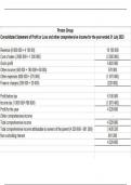
It is important for the CB to forecast how the economy will respond in the future, to current changes
in the IR
,The dynamic IS curve captures that there is a lag between a change in IR and a change in investment
Supply – SRAS
Phillips’s curve – describes the supply side in the SR
ERU: equilibrium relative unemployment
The price setting and wage setting supply curves come together for the PC but we need to assume
that productivity is constant, that prices are flexible (so, price setters change their prices in line with
wage demand)
We will assume that wage setting is describe by an efficiency wage model.
The PC describes the relationship between price inflation, and the real side of the economy.
Real side of the economy in terms of output
But we can also describe the real side in terms of unemployment.
The formular shows that inflation (pie t) depends on expected inflation and the output gap
Expected inflation assumes that peoples inflation expectations are backward looking (so, people
expect inflation to be the same as it was last period) pie t - 1
Output gap yt – ye
The CB is satisfied when y = ye
The output gap is hard to measure as it is hard to know what
the stable equilibrium for the economy is at a point in time.
Equilibrium unemployment is easier to measure and see how
it tends towards an equilibrium level.
Output and unemployment are negatively related and the PC
is a negatively sloped relation between unemployment and
inflation.
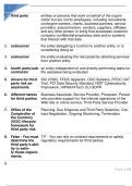
In the 3-equation model, the labour market isn’t fully flexible because of efficiency wages. Firms set
the wage, w, above the firm’s reservation wage (as they want to induce working instead of shirking).
Workers in this economy get an unemployment benefit if they don’t work. And because they don’t
exert effort, where effort causes disutility.
The wage setting curve describes the behaviour of workers that shows, to increase the labour supply
(employment), the real wage has to rise higher and higher.
, In the WS-PS
model,
wages at
equilibrium
unemployment are higher
than workers would be
willing to accept; this
means there is involuntary
unemployment.
, When unemployment is high, the cost of job loss is high (as it is hard to find a job if you get laid
off), so a low wage (above the opportunity cost of working) must be paid for the workers to supply
their labour.
Whereas if unemployment is low, it is easy to find a job if you get laid off, so to increase effort firms
would have to pay a higher wage premium over the opportunity cost of working.
These relationships form the wage-setting curve.
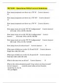
What happens to wage setting as employment and output deviate from their equilibrium levels.
impact of a demand shock: Ne is the equilibrium
level of employment. A positive shock
employment rises above equilibrium level (NH)
induced by a positive output gap the cost of job
loss falls, so a higher wage is needed to induce
workers to work.
The higher wage leads to upward pressure on
nominal wages
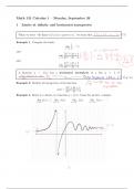
Impact of a supply shock: WS and PS are the only source of supply shocks in the 3-equation model. A
supply shock is represented by a shift in the WS or PS curve.
What causes the WS to shift: shift in ws, ws shift
Wage push factors (zw) shifts the WS curve down
Efficiency wage factors:
- Reducing the unemployment benefit would reduce the opportunity cost of working and lead
to an equivalent fall shift in the WS curve.
- Improving the working conditions raises the cost of unemployment by increasing the
benefits of being in a job, so it would lead to a fall in the WS curve.
Union related:
- Less legal protection for unions
- Weaker union power
- Unions exercise bargaining constraint lower union markup
Wage and price setting
1. IS curve – dynamics IS curve
2. Phillips curve PC – inflation determination, wage setting, price setting
3. Monetary response curve MR
The dynamic IS curve – aggregate demand
Demand (Yd) comes from consumers, firms and the government these
all sum to give aggregate demand
C (consumer spending), I (firms investment), G (government spending)
C0 autonomous consumption (happens no matter the level of income) - consumer
C1 as income rises, consumption rises too (MPC) ; high MPC = flatter IS curve as it increases size of
multiplier. A higher multiplier means that a given change in real interest rate r will lead to a larger change in real output y
I total income, y, minus tax, t (1-t)y – consumer
a0 autonomous investment (happens no matter what the cost of investment/ finance – invest
r the real IR that firms must pay to borrow - invest
a1 interest sensitivity of investment changes in spending/ consumption SHIFTS is curve
a1r each time r goes up, investment goes down it doesn’t change the slope
G government spending (demand rises with government spending) – gov. spending is exogenous
as it doesn’t depend on any other factor
Everything demanded must be supplied
y production/output
IS equation: A – ar
The IS equation assumes the real rate only negatively
effects investment, and it has no impact on consumer
spending by assumption, and it isn’t thought to effect
government spending y assumption
Slope of the IS curve
High r low investment low y
Low r high investment high y
High multiplier/high sensitivity (a1) = flat IS curve
Anything that raises the multiplier will reduce the slope of the IS
curve. A higher tax rate increases the size of the multiplier
Shifts of IS curve
Causes by changes in c0, a0, or gov. spending
How much it shifts: Shifts by the multiplier x change in spending
It is important for the CB to forecast how the economy will respond in the future, to current changes
in the IR
,The dynamic IS curve captures that there is a lag between a change in IR and a change in investment
Supply – SRAS
Phillips’s curve – describes the supply side in the SR
ERU: equilibrium relative unemployment
The price setting and wage setting supply curves come together for the PC but we need to assume
that productivity is constant, that prices are flexible (so, price setters change their prices in line with
wage demand)
We will assume that wage setting is describe by an efficiency wage model.
The PC describes the relationship between price inflation, and the real side of the economy.
Real side of the economy in terms of output
But we can also describe the real side in terms of unemployment.
The formular shows that inflation (pie t) depends on expected inflation and the output gap
Expected inflation assumes that peoples inflation expectations are backward looking (so, people
expect inflation to be the same as it was last period) pie t - 1
Output gap yt – ye
The CB is satisfied when y = ye
The output gap is hard to measure as it is hard to know what
the stable equilibrium for the economy is at a point in time.
Equilibrium unemployment is easier to measure and see how
it tends towards an equilibrium level.
Output and unemployment are negatively related and the PC
is a negatively sloped relation between unemployment and
inflation.
In the 3-equation model, the labour market isn’t fully flexible because of efficiency wages. Firms set
the wage, w, above the firm’s reservation wage (as they want to induce working instead of shirking).
Workers in this economy get an unemployment benefit if they don’t work. And because they don’t
exert effort, where effort causes disutility.
The wage setting curve describes the behaviour of workers that shows, to increase the labour supply
(employment), the real wage has to rise higher and higher.
, In the WS-PS
model,
wages at
equilibrium
unemployment are higher
than workers would be
willing to accept; this
means there is involuntary
unemployment.
, When unemployment is high, the cost of job loss is high (as it is hard to find a job if you get laid
off), so a low wage (above the opportunity cost of working) must be paid for the workers to supply
their labour.
Whereas if unemployment is low, it is easy to find a job if you get laid off, so to increase effort firms
would have to pay a higher wage premium over the opportunity cost of working.
These relationships form the wage-setting curve.
What happens to wage setting as employment and output deviate from their equilibrium levels.
impact of a demand shock: Ne is the equilibrium
level of employment. A positive shock
employment rises above equilibrium level (NH)
induced by a positive output gap the cost of job
loss falls, so a higher wage is needed to induce
workers to work.
The higher wage leads to upward pressure on
nominal wages
Impact of a supply shock: WS and PS are the only source of supply shocks in the 3-equation model. A
supply shock is represented by a shift in the WS or PS curve.
What causes the WS to shift: shift in ws, ws shift
Wage push factors (zw) shifts the WS curve down
Efficiency wage factors:
- Reducing the unemployment benefit would reduce the opportunity cost of working and lead
to an equivalent fall shift in the WS curve.
- Improving the working conditions raises the cost of unemployment by increasing the
benefits of being in a job, so it would lead to a fall in the WS curve.
Union related:
- Less legal protection for unions
- Weaker union power
- Unions exercise bargaining constraint lower union markup
Wage and price setting