LECTURE 1 : GAME THEORY AND COMPETITION
H1. Game Theory
Game theory is a mathematical tool used to represent strategic interactions in a treatable way.
→ Representation of agents’ goals, information and capabilities
→ Goals:
- Predict outcomes when conflicting goals
- Understand what factors can give an edge to different players
- Identify pitfalls
Agents are individually rational:
→ They have rational preferences
- They can rank outcomes (most favourite -> least favourite)
→ Payoff-maximizing
- Strategy chosen to achieve highest payoff for themselves
THREE MAIN CATEGORIES OF GAMES
1. Strategic
Example: Rock-Paper-Scissor
I Static
g One-shot game
g Simultaneous choice: players choose w/o knowing other’s choice
II Complete information
g All players know capabilities of every other player
g All players know consequences of every combination
Games involve quantifiable risk. If all the possible outcomes are known and occur with a known probability
distribution, we call this risk “uncertainty".
→ If I buy a stock of Meta today, I don’t know the price it will have tomorrow, but
I can form expectations and quantify the likelihood of different price swings.
However, sometimes a player may know something that others don’t. Then we say that players have
asymmetric information
→ Mark Zuckerberg secretly sets on fire the Meta headquarters and now he is short selling Meta stocks. I
know that he knows more than me, but I don’t know what he knows.
Strategic games allow for uncertainty, but not asymmetric information.
Strategic games are described by:
→ Set of players: P = {Player1, Player2}
→ Set of actions for each player: AP1 = {Defect, Cooperate}, AP2 = {Defect, Cooperate}
→ Player’s payoff functions:
1
, (−1, −1) if (Defect, Defect)
⎧
(+5, −5) if (Defect, Cooperate)
(Payoff P1, Payoff P2) =
⎨(−5, +5) if (Cooperate, Defect)
⎩(+3, +3) if (Cooperate, Cooperate)
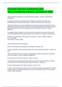
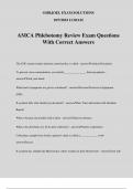
• Rows represent the actions of one player
(e.g., P1 choosing between D, C, or H). (p1, p2)
• Columns represent the actions of the other
player (e.g., P2 choosing between X, Y, or T).
• Each cell contains the payoff for both players
corresponding to their chosen actions
• Payoffs reflect players' preferences for
outcomes, while action profiles indicate the actions chosen by each player.
For instance, < C, Y > and < H, T > may yield the same payoffs (3, 3), making players indifferent
between these outcomes.
An equilibrium in dominant strategy is a very strong notion, only relies on player’s rationality.
→ Pro: it’s the only possible outcome so very reliable
→ Con: most games don’t have one
A Nash Equilibrium (NE) is an action profile such that none of the players can increase their
payoff by choosing a different strategy, taking the other player’s strategies for given.
→ Each player is playing their best-response to the other players’ strategies (indifferent)
→ Nothing optimal, it’s a resting point
→ Pure strategy NE: Each player's chosen strategy is the best response to the other player's strategy, with
no incentive to change unilaterally.
→ Mixed strategy NE: Players randomize their actions based on probabilities <p,q>, with each player's
strategy being optimal given the others', and no player can improve their expected payoff by changing their
strategy alone. Every strategic game has at least one equilibrium in mixed strategies.
2. Extensive
Example: Chess, Monopoly
g Analyses decision-making in situations of sequential interaction, where players
make choices at different points in time, often represented through decision
trees.
3. Sequential and Bayesian
Example: Sealed-bid auction (Bayesian), poker (sequential)
g Explores strategic interactions where players make decisions sequentially,
with Bayesian elements incorporated to account for uncertainty and
incomplete information about the other players' actions or types.
2
,H2. Demand, Monopoly and Competition
Demand function tells us how many units of a product are
purchased by consumers, depending on its price
!"
→ !# shows decrease/increase of units sold for small
increment/reduction in the price. For normal goods à always negative
→ Economists use price elasticity of demand
∆"
" !"(#) #
𝜀(𝑝) = ∆# = !#
∗ "(#)
#
∆" ∆#
"
is the percentage change in q and #
is the percentage change in p
g Always negative (for normal goods). Describes the ability/willingness of consumers to substitute
consumption with another good (or not spend).
g |𝜀| = 1 : if price reduces (increases) by 5%, then quantity increases (reduces) by the same
percentage amount
g |𝜀| < 1 : Demand is inelastic ⇒ ∆𝑝 > ∆𝑞
g |𝜀| > 1 : Demand is elastic ⇒ ∆𝑝 < ∆𝑞
LINEAIR DEMAND
g Represents the relationship between quantity demand 𝑞 and price 𝑝 as 𝑞(𝑝) = 𝑎 – 𝑏𝑝.
g 𝒂 signifies the quantity demanded when the price is infinitesimally small.
g The slope of the demand curve is constant and equals to 𝒃.
g However, the elasticity of demand is not constant.
INVERSE DEMAND
g Inverse demand can be expressed as 𝑝(𝑞), where p represents price and q represents quantity
demanded.
' )
g For linear inverse demand, the equation is: 𝑝 = 𝐴 − 𝐵 ∗ 𝑞 with ( = 𝐴, ( = 𝐵
g 𝐴 represents the maximum willingness to pay among consumers.
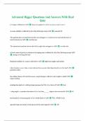
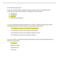
PERFECT COMPETITION
Does not exist, useful as benchmark
g In perfect competition, the market consists of many small firms, each
acting as a price taker, price equals marginal costs
g The inverse demand curve is a horizontal line at price 𝑝̄, indicating
that consumers are willing to buy any quantity at or below this price.
g There are infinitely many firms willing to supply at the price 𝑝̄.
g Price elasticity at any quantity 𝑞 is infinite.
3
, g Price-Taking Firm
- Each firm observes the market price 𝑝̄ and aims to maximize
profit.
- It produces the quantity that maximizes its profit, considering its
cost function 𝐶(𝑞).
- The firm's profit-maximizing condition is given by the equation
𝑝̄ = 𝐶′(𝑞), where 𝐶′(𝑞) represents the marginal cost.
- Price-taking firms can make profits if the market price is
sufficiently high, but in the long run, profits tend to zero due to
free entry, as prices decrease to the minimum of the Average
Total Cost Curve (ATC).
Conclusion:
Perfect competition serves as a benchmark model, although it may not exist in reality.
Price-taking firms, coupled with free entry, lead to zero profits in the long run, making it an unattractive
market for new entrants but beneficial for consumers.
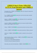
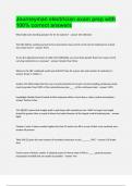
MONOPOLISTS PROBLEM: PRICE-SETTING
g The monopolist faces a single-agent problem, where it aims to maximize profits by setting prices.
g The monopolist observes a downward-sloping demand curve represented by the function 𝑞(𝑝),
indicating the quantity demanded at various price levels.
g It can produce its product at a cost determined by the cost function 𝐶(𝑞).
g The monopolist's objective is to choose the price (or quantity) that maximizes its profits ∏.
g Mathematically, this is expressed as maximizing the profit function
𝑚𝑎𝑥{𝛱(𝑝) = 𝑝 ∗ 𝑞(𝑝) − 𝐶(𝑞(𝑝))}
Elaboration:
*"(#) *+,"(#)- *"(#)
0 = 𝑞(𝑝) + 𝑝 ∗ − ∗
*# *" *#
*"(#)
𝑞(𝑝) = − (𝑝 − 𝐶 . (𝑞))
*#
*"(#) /) "(#) ,#/+ $ (")-
−J K =
*# # LMNMO
#
Lerner Index (%Markup)
) ) /)
J1 + 0 K 𝑝 = 𝐶 . (𝑞(𝑝)) 𝑝 = J1 + 0 K 𝐶 . (𝑞(𝑝))
→ LMMMMMMNMMMMMMO
è A monopolist prices above marginal cost, how much depends on 𝜺 (see numerical example in slides)
IMPERFECT COMPETITION: BERTRAND DUOPOLY
1. Conditional demand
We introduce 1 competitor à now it’s a 2-player game
g Firm 1 & 2 produce a homogeneous product
g Both firms have same 𝐶(𝑞)
g Each firm, 𝑖 ∈ {1, 2}, chooses its own price 𝑝1 simultaneously
g Consumers have a demand 𝑞 = 𝑎 − 𝑏𝑝 , but only buy from the cheapest firm
g If prices are equal, consumers split their purchases equally between the two firms.
g Firms only produce (and thus incur costs) when and if units are sold.
g 𝐶 . (𝑞) = 𝑐
4
, So, firm's 𝑖 demand given the own price 𝑝1 and the competitor's 𝑝/1 is as follows:
0 if 𝑝1 > 𝑝/1
𝑞1 (𝑝1 ∣ 𝑝/1 ) = W(𝑎 − 𝑏𝑝1 )/2 if 𝑝1 = 𝑝/1
(𝑎 − 𝑏𝑝1 ) if 𝑝1 < 𝑝/1
(see numerical example in slides)
Conditional Profits:
g The firm's profits vary based on whether its own price is greater than, equal to, or less than its
competitor's price
g If firm 1 sets a price above the monopoly price, profits are negative if firm 2's price is less than the
cost.
g When both firms set prices equal to the monopoly price, profits are half of the monopoly profits.
g Undercutting by either firm can lead to higher profits, even close to the full monopoly profits.
g For Firm 1, setting a price below the monopoly price but above its cost results in positive profits.
g Reaching optimal pricing involves strategic considerations, including undercutting and stopping
points for price adjustments.
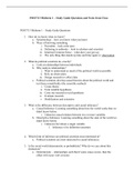
2. Reaction function
g Best response to any price 𝑝/) (competitor price)
3. Nash Equilibrium
𝑝1 < 𝑐 à firms make loss
𝑝1 > 𝑝2 à 1 firm wants to undercut
𝑐 < 𝑝1 < 𝑝2 à either firm can undercut & take positive profits
g Only equilibrium is 𝒑𝟏 = 𝒑𝟐 = 𝒄
Intersection of R-curves is always Nash Equilibrium
Competitive Outcome:
g Two firms can achieve a competitive outcome by pricing at marginal cost 𝑝 = 𝑐 = 𝐶′
g Market concentration alone doesn't necessarily lead to market power = Bertrand's Paradox
This paradox suggests that even with only two firms, they can produce the same output as perfect
competition and earn zero profit.
g Despite the theoretical expectation of zero profits in perfect competition, many firms do make profits
in reality.
g Reasons for this include:
o Increasing marginal costs, which can lead to short-term profits even in perfect competition.
o Capacity constraints, where firms may not be able to immediately scale up production to meet demand.
o Search or information frictions, as consumers may not quickly find the cheapest option.
5
H1. Game Theory
Game theory is a mathematical tool used to represent strategic interactions in a treatable way.
→ Representation of agents’ goals, information and capabilities
→ Goals:
- Predict outcomes when conflicting goals
- Understand what factors can give an edge to different players
- Identify pitfalls
Agents are individually rational:
→ They have rational preferences
- They can rank outcomes (most favourite -> least favourite)
→ Payoff-maximizing
- Strategy chosen to achieve highest payoff for themselves
THREE MAIN CATEGORIES OF GAMES
1. Strategic
Example: Rock-Paper-Scissor
I Static
g One-shot game
g Simultaneous choice: players choose w/o knowing other’s choice
II Complete information
g All players know capabilities of every other player
g All players know consequences of every combination
Games involve quantifiable risk. If all the possible outcomes are known and occur with a known probability
distribution, we call this risk “uncertainty".
→ If I buy a stock of Meta today, I don’t know the price it will have tomorrow, but
I can form expectations and quantify the likelihood of different price swings.
However, sometimes a player may know something that others don’t. Then we say that players have
asymmetric information
→ Mark Zuckerberg secretly sets on fire the Meta headquarters and now he is short selling Meta stocks. I
know that he knows more than me, but I don’t know what he knows.
Strategic games allow for uncertainty, but not asymmetric information.
Strategic games are described by:
→ Set of players: P = {Player1, Player2}
→ Set of actions for each player: AP1 = {Defect, Cooperate}, AP2 = {Defect, Cooperate}
→ Player’s payoff functions:
1
, (−1, −1) if (Defect, Defect)
⎧
(+5, −5) if (Defect, Cooperate)
(Payoff P1, Payoff P2) =
⎨(−5, +5) if (Cooperate, Defect)
⎩(+3, +3) if (Cooperate, Cooperate)
• Rows represent the actions of one player
(e.g., P1 choosing between D, C, or H). (p1, p2)
• Columns represent the actions of the other
player (e.g., P2 choosing between X, Y, or T).
• Each cell contains the payoff for both players
corresponding to their chosen actions
• Payoffs reflect players' preferences for
outcomes, while action profiles indicate the actions chosen by each player.
For instance, < C, Y > and < H, T > may yield the same payoffs (3, 3), making players indifferent
between these outcomes.
An equilibrium in dominant strategy is a very strong notion, only relies on player’s rationality.
→ Pro: it’s the only possible outcome so very reliable
→ Con: most games don’t have one
A Nash Equilibrium (NE) is an action profile such that none of the players can increase their
payoff by choosing a different strategy, taking the other player’s strategies for given.
→ Each player is playing their best-response to the other players’ strategies (indifferent)
→ Nothing optimal, it’s a resting point
→ Pure strategy NE: Each player's chosen strategy is the best response to the other player's strategy, with
no incentive to change unilaterally.
→ Mixed strategy NE: Players randomize their actions based on probabilities <p,q>, with each player's
strategy being optimal given the others', and no player can improve their expected payoff by changing their
strategy alone. Every strategic game has at least one equilibrium in mixed strategies.
2. Extensive
Example: Chess, Monopoly
g Analyses decision-making in situations of sequential interaction, where players
make choices at different points in time, often represented through decision
trees.
3. Sequential and Bayesian
Example: Sealed-bid auction (Bayesian), poker (sequential)
g Explores strategic interactions where players make decisions sequentially,
with Bayesian elements incorporated to account for uncertainty and
incomplete information about the other players' actions or types.
2
,H2. Demand, Monopoly and Competition
Demand function tells us how many units of a product are
purchased by consumers, depending on its price
!"
→ !# shows decrease/increase of units sold for small
increment/reduction in the price. For normal goods à always negative
→ Economists use price elasticity of demand
∆"
" !"(#) #
𝜀(𝑝) = ∆# = !#
∗ "(#)
#
∆" ∆#
"
is the percentage change in q and #
is the percentage change in p
g Always negative (for normal goods). Describes the ability/willingness of consumers to substitute
consumption with another good (or not spend).
g |𝜀| = 1 : if price reduces (increases) by 5%, then quantity increases (reduces) by the same
percentage amount
g |𝜀| < 1 : Demand is inelastic ⇒ ∆𝑝 > ∆𝑞
g |𝜀| > 1 : Demand is elastic ⇒ ∆𝑝 < ∆𝑞
LINEAIR DEMAND
g Represents the relationship between quantity demand 𝑞 and price 𝑝 as 𝑞(𝑝) = 𝑎 – 𝑏𝑝.
g 𝒂 signifies the quantity demanded when the price is infinitesimally small.
g The slope of the demand curve is constant and equals to 𝒃.
g However, the elasticity of demand is not constant.
INVERSE DEMAND
g Inverse demand can be expressed as 𝑝(𝑞), where p represents price and q represents quantity
demanded.
' )
g For linear inverse demand, the equation is: 𝑝 = 𝐴 − 𝐵 ∗ 𝑞 with ( = 𝐴, ( = 𝐵
g 𝐴 represents the maximum willingness to pay among consumers.
PERFECT COMPETITION
Does not exist, useful as benchmark
g In perfect competition, the market consists of many small firms, each
acting as a price taker, price equals marginal costs
g The inverse demand curve is a horizontal line at price 𝑝̄, indicating
that consumers are willing to buy any quantity at or below this price.
g There are infinitely many firms willing to supply at the price 𝑝̄.
g Price elasticity at any quantity 𝑞 is infinite.
3
, g Price-Taking Firm
- Each firm observes the market price 𝑝̄ and aims to maximize
profit.
- It produces the quantity that maximizes its profit, considering its
cost function 𝐶(𝑞).
- The firm's profit-maximizing condition is given by the equation
𝑝̄ = 𝐶′(𝑞), where 𝐶′(𝑞) represents the marginal cost.
- Price-taking firms can make profits if the market price is
sufficiently high, but in the long run, profits tend to zero due to
free entry, as prices decrease to the minimum of the Average
Total Cost Curve (ATC).
Conclusion:
Perfect competition serves as a benchmark model, although it may not exist in reality.
Price-taking firms, coupled with free entry, lead to zero profits in the long run, making it an unattractive
market for new entrants but beneficial for consumers.
MONOPOLISTS PROBLEM: PRICE-SETTING
g The monopolist faces a single-agent problem, where it aims to maximize profits by setting prices.
g The monopolist observes a downward-sloping demand curve represented by the function 𝑞(𝑝),
indicating the quantity demanded at various price levels.
g It can produce its product at a cost determined by the cost function 𝐶(𝑞).
g The monopolist's objective is to choose the price (or quantity) that maximizes its profits ∏.
g Mathematically, this is expressed as maximizing the profit function
𝑚𝑎𝑥{𝛱(𝑝) = 𝑝 ∗ 𝑞(𝑝) − 𝐶(𝑞(𝑝))}
Elaboration:
*"(#) *+,"(#)- *"(#)
0 = 𝑞(𝑝) + 𝑝 ∗ − ∗
*# *" *#
*"(#)
𝑞(𝑝) = − (𝑝 − 𝐶 . (𝑞))
*#
*"(#) /) "(#) ,#/+ $ (")-
−J K =
*# # LMNMO
#
Lerner Index (%Markup)
) ) /)
J1 + 0 K 𝑝 = 𝐶 . (𝑞(𝑝)) 𝑝 = J1 + 0 K 𝐶 . (𝑞(𝑝))
→ LMMMMMMNMMMMMMO
è A monopolist prices above marginal cost, how much depends on 𝜺 (see numerical example in slides)
IMPERFECT COMPETITION: BERTRAND DUOPOLY
1. Conditional demand
We introduce 1 competitor à now it’s a 2-player game
g Firm 1 & 2 produce a homogeneous product
g Both firms have same 𝐶(𝑞)
g Each firm, 𝑖 ∈ {1, 2}, chooses its own price 𝑝1 simultaneously
g Consumers have a demand 𝑞 = 𝑎 − 𝑏𝑝 , but only buy from the cheapest firm
g If prices are equal, consumers split their purchases equally between the two firms.
g Firms only produce (and thus incur costs) when and if units are sold.
g 𝐶 . (𝑞) = 𝑐
4
, So, firm's 𝑖 demand given the own price 𝑝1 and the competitor's 𝑝/1 is as follows:
0 if 𝑝1 > 𝑝/1
𝑞1 (𝑝1 ∣ 𝑝/1 ) = W(𝑎 − 𝑏𝑝1 )/2 if 𝑝1 = 𝑝/1
(𝑎 − 𝑏𝑝1 ) if 𝑝1 < 𝑝/1
(see numerical example in slides)
Conditional Profits:
g The firm's profits vary based on whether its own price is greater than, equal to, or less than its
competitor's price
g If firm 1 sets a price above the monopoly price, profits are negative if firm 2's price is less than the
cost.
g When both firms set prices equal to the monopoly price, profits are half of the monopoly profits.
g Undercutting by either firm can lead to higher profits, even close to the full monopoly profits.
g For Firm 1, setting a price below the monopoly price but above its cost results in positive profits.
g Reaching optimal pricing involves strategic considerations, including undercutting and stopping
points for price adjustments.
2. Reaction function
g Best response to any price 𝑝/) (competitor price)
3. Nash Equilibrium
𝑝1 < 𝑐 à firms make loss
𝑝1 > 𝑝2 à 1 firm wants to undercut
𝑐 < 𝑝1 < 𝑝2 à either firm can undercut & take positive profits
g Only equilibrium is 𝒑𝟏 = 𝒑𝟐 = 𝒄
Intersection of R-curves is always Nash Equilibrium
Competitive Outcome:
g Two firms can achieve a competitive outcome by pricing at marginal cost 𝑝 = 𝑐 = 𝐶′
g Market concentration alone doesn't necessarily lead to market power = Bertrand's Paradox
This paradox suggests that even with only two firms, they can produce the same output as perfect
competition and earn zero profit.
g Despite the theoretical expectation of zero profits in perfect competition, many firms do make profits
in reality.
g Reasons for this include:
o Increasing marginal costs, which can lead to short-term profits even in perfect competition.
o Capacity constraints, where firms may not be able to immediately scale up production to meet demand.
o Search or information frictions, as consumers may not quickly find the cheapest option.
5