RSM, Erasmus University
Msc BIM 2021 - 2022
Kathleen Gaillot
BM06BIM • 4 EC
BIM Research Methods
Summary Notes/imagery based on lectures
Discovering Statistics using R. by Field A. ISBN: 978-1-4462-0045-2
Social Science Research: Principles, Methods, and Practices. by
1
Bhattacherjee A. ISBN: 978-1475146127
Mastering Metrics: The Path from Cause to Effect. by Angrist J. ISBN:
978-0-691-15284-4
, Table of Contents
Session 1: Econometrics I .............................................. 1 4.2.1 Experiments: Gold Standard of Causal
1.1 Plotting your Data............................................... 1 Inference ........................................................... 25
1.1.1 Scatterplot .................................................. 1 4.2.2 Four types of Experiments........................ 25
1.1.2 Histograms.................................................. 2 4.3 Experimental Designs ....................................... 26
1.1.3 Boxplots ...................................................... 2 4.3.1 Theoretical & Empirical Plane .................. 26
1.1.4 Bar Charts ................................................... 3 4.3.2 Reliability & Validity ................................. 26
1.2 Terminology ........................................................ 3 4.3.3 Experimental Designs ............................... 27
1.3 Central Limit Theorem ........................................ 5 4.3.4 Conducting Experiments: The Steps ......... 27
1.3.1 Normal Distribution, Standard Deviation & Session 5: Obtaining Data Using Surveys.....................32
Probability ........................................................... 6 5.1 Method of Choice ............................................. 32
1.3.2 Type I & Type II Errors ................................ 7 5.1.1 Use of a Survey ......................................... 32
1.4 Hypotheses ......................................................... 7 5.2 Sample Strategy ................................................ 32
1.4.1 Assessing Normality ................................... 7 5.2.1 What is Your Population? ......................... 32
Session 2: Econometrics II ............................................. 8 5.2.2 How to Sample?........................................ 33
2.1 Simple Linear Regressions .................................. 8 5.3 Survey Design ................................................... 33
2.1.1 Ordinary Least Squares (OLS) Regression... 8 5.3.1 Concepts Into Measurable Variables........ 33
2.1.2 Testing the Model: R2 ................................. 8 5.3.2 Abstract Constructs .................................. 34
2.2 Multiple Linear Regression ............................... 10 5.3.3 Types of Questions to Avoid..................... 36
2.2.1 OLS (ordinary least square) Assumptions 10 5.3.4 Survey Design ........................................... 37
2.3 T-Test ................................................................ 11 5.3.5 Qualtrics Overview ................................... 38
2.3.2 The Dependent T-Test .............................. 11 5.3.6 Survey Design: Pre-Test/Experts .............. 39
2.3.1 The independent T-Test ........................... 11 5.4 Data Collection ................................................. 39
2.4 Effect Size ......................................................... 12 5.4.1 Administering Survey ............................... 40
2.4.1 Reporting Results ..................................... 12 5.4.2 Survey Structure ....................................... 40
2.5 Logistic Regression ........................................... 12 5.4.3 Data Analysis ............................................ 41
2.6 Assessing Predictors ......................................... 13 5.4.4 Other Types of Variable Analysis .............. 42
2.7 Assessing the Model ......................................... 14 5.4.5 Possible Threats........................................ 44
2.7.1 Unique Model Problems........................... 15 Session 6: Econometrics IV ..........................................45
Session 3: Case Study Research ................................... 16 6.1 Experiments for Investigating Causal
3.1 Case Study as Research Strategy ...................... 16 Hypotheses ............................................................. 45
3.1.1 Theory Versus Empirical Reality ............... 16 6.1.1 Quasi-Experiment in the Field .................. 45
3.1.2 Case Study Method (Yin 2003) ................. 17 6.2 Difference-in-Difference (DiD) Strategy ........... 45
3.2 Designing Case Studies ..................................... 17 6.2.1 Common Trend Assumption..................... 46
3.2.1 Components of Research Design.............. 17 6.2.2 Stable Unit Treatment Value Assumption
3.3 Conducting Case Studies .................................. 18 (SUTVA).............................................................. 47
3.3.1 Preparing for Data Collection ................... 18 6.2.3 Conditional Independence Assumption
3.3.2 Collecting Evidence................................... 18 (CIA) ................................................................... 47
3.4 Analysing Case Study Evidence......................... 19 6.3 Apply the Difference-in-Difference Method .... 47
3.5 Reporting Case Studies ..................................... 19 6.3.1 Difference-in-Difference (DiD)
3.6 Thesis Case Study Example ............................... 19 Regression: ........................................................ 47
Session 4: Econometrics III .......................................... 24 6.3.2 What do the Coefficients Tell us?............. 48
4.1Pitfalls of Observational Data ............................ 24 6.3.3 Fixed Effects.............................................. 51
4.1.1 Correlation & Causation ........................... 24 6.3.4 DiD Recap ................................................. 51
4.1.2 Biases ........................................................ 24 Examination Information .............................................52
4.2 Randomized Experiments ................................. 25 7.1 Evaluation Info .................................................. 52
7.2 Exam Samples ................................................... 52
Note: use CTRL + F for quick navigation / finding keywords.
ii
, Learning Objectives
Describe the basic research methodologies in Explain how to decide on a research methodology in the
the BIM field domain of empirical research
Understand how to design a survey Clean, organize and analyse data in R
Display data in various graphs Interpret probabilities and random variables
Discuss and explain research hypotheses Perform basic univariate multivariate econometric analyses
Justify certain research methods for the Evaluate the difference in performance of different statistical
research question at hand methods and discuss advantages and drawbacks of methods
Session 1: Econometrics I
Literature: Field et al. (2021) Ch.2 & 5
1.1 Plotting your Data
How to present data clearly?
Show the data;
Induce the reader to think about the data being presented (rather than some other aspect of the graph);
Avoid distorting the data;
Present many numbers with minimum ink;
Make large data sets (assuming you have one) coherent);
Encourage the reader to compare different pieces of data;
Reveal the data.
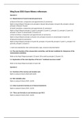
1.1.1 Scatterplot
Simple scatterplot with Smooth Line Simple scatterplot with Regression Line
scatter <- ggplot(examData, aes(Anxiety, Exam)) scatter <- ggplot(examData, aes(Anxiety, Exam))
scatter + geom_point() + geom_smooth() lab(x = scatter + geom_point() + geom_smooth(method =
"Exam Anxiety", y = "Exam Performance %") "lm", colour = "Red")+ labs(x = "Exam Anxiety",
y = "Exam Performance %")
Scatter plots are useful to see the general tendency of your data (is it linear? Do I see an obvious trend?)
1
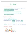
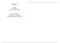
,Grouped Scatterplots with Regression Lines
scatter <- ggplot(examData, aes(Anxiety, Exam,
colour = Gender)) scatter + geom_point() +
geom_smooth(method = "lm", aes(fill = Gender),
alpha = 0.1) + labs(x = "Exam Anxiety", y = "Exam
Performance %", colour = "Gender")
The correlation between male anxiety and male performance
is stronger (vs woman).
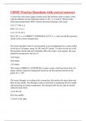
1.1.2 Histograms
The score (x-axis) festivalHistogram <-
o The frequency (y-axis) ggplot(festivalData,
Histograms help us to identify: aes(day1))
festivalHistogram +
o The shape of the distribution geom_histogram(binwidt
o Skew the mode of the distribution is either: h = 0.4 ) + labs(x =
Left (positive skew) or "Hygiene (Day 1 of
Festival)", y =
Right (negative skew) "Frequency")
o Kurtosis (when your distribution is very pointy)
o Spread or variation in scores shows the skewness
Unusual scores
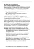
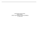
1.1.3 Boxplots
The box shows:
• The median (middle score when numbers are ordered)
• The upper and lower quartile
• The limits within which the middle 50% of scores lie.
• The limits within which the top and bottom 25% of scores lie
The whiskers show:
• The range of scores
• The limits within which the top and bottom 25% of scores lie
Quartiles
o The three values that split the sorted data into four equal parts
o Second quartile = median
o Lower quartile = median of lower half of the data
o Upper quartile = median of upper half of the data
Good to find outliers and how your data is distributed →
2
, 1.1.4 Bar Charts
This is a good chart for mean comparison. The vertical lines around the mean are the confidence intervals.
The error bar sticks out from the bar like a whisker. It displays the precision of the mean in one of three ways:
(1) Confidence interval (usually 95%), (2) Standard deviation, (3) Standard error of the mean
Bar Chart: One Dependent Variable:
Step 1: bar <- ggplot(ChickFlick, aes(film, arousal)) bar +
stat_summary(fun.y = mean, geom = "bar", fill = "White", colour =
"Black")
Step 2: …stat_summary(fun.data = mean_cl_normal, geom = "pointrange") …+
labs(x = "Film", y = "Mean Arousal")
Step 3:
bar + stat_summary(fun.y = mean, geom = "bar", fill = "White", colour
= "Black") + stat_summary(fun.data = mean_cl_normal, geom =
"pointrange") + labs(x = "Film", y = "Mean Arousal")
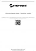
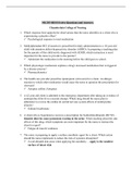
Bar Chart: Two Independent Variables:
bar + stat_summary(fun.y = mean, geom = "bar",
position="dodge") +
stat_summary(fun.data = mean_cl_normal, geom = "errorbar",
position = position_dodge(width = 0.90), width = 0.2) + labs(x
= "Film", y = "Mean Arousal", fill = "Gender")
Men enjoy Bridget Jones more (on average) than women. Looking at the
confidence intervals, the means are statistically different for Bridget Jones
and not for Momento.
Two Independent Variables in Separate Panels
bar <- ggplot(chickFlick, aes(film, arousal, fill = film))
bar + stat_summary(fun.y = mean, geom = "bar") +
stat_summary(fun.data
= mean_cl_normal, geom = "errorbar", width = 0.2) + facet_wrap( ~
gender) + labs(x = "Film", y = "Mean Arousal")
1.2 Terminology
Hypothesis Independent Variable Dependent Variable
o Statement of o The proposed cause o The proposed effect
cause and o A predictor variable o An outcome variable
effect o A manipulated variable (in experiments) o Measured not manipulated (in experiments)
o ‘The early bird o Whether a bird wakes up early or late to go get the o Whether the bird catches the worm or not
catches the worms o Observed
worm’
Population Sample
o The collection of units (be they people, plankton, plants, cities, suicidal o A smaller (but hopefully representative)
authors, etc.) to which we want to generalize a set of findings or a collection of units from a population used to
statistical model. determine truths about that population.
3
Msc BIM 2021 - 2022
Kathleen Gaillot
BM06BIM • 4 EC
BIM Research Methods
Summary Notes/imagery based on lectures
Discovering Statistics using R. by Field A. ISBN: 978-1-4462-0045-2
Social Science Research: Principles, Methods, and Practices. by
1
Bhattacherjee A. ISBN: 978-1475146127
Mastering Metrics: The Path from Cause to Effect. by Angrist J. ISBN:
978-0-691-15284-4
, Table of Contents
Session 1: Econometrics I .............................................. 1 4.2.1 Experiments: Gold Standard of Causal
1.1 Plotting your Data............................................... 1 Inference ........................................................... 25
1.1.1 Scatterplot .................................................. 1 4.2.2 Four types of Experiments........................ 25
1.1.2 Histograms.................................................. 2 4.3 Experimental Designs ....................................... 26
1.1.3 Boxplots ...................................................... 2 4.3.1 Theoretical & Empirical Plane .................. 26
1.1.4 Bar Charts ................................................... 3 4.3.2 Reliability & Validity ................................. 26
1.2 Terminology ........................................................ 3 4.3.3 Experimental Designs ............................... 27
1.3 Central Limit Theorem ........................................ 5 4.3.4 Conducting Experiments: The Steps ......... 27
1.3.1 Normal Distribution, Standard Deviation & Session 5: Obtaining Data Using Surveys.....................32
Probability ........................................................... 6 5.1 Method of Choice ............................................. 32
1.3.2 Type I & Type II Errors ................................ 7 5.1.1 Use of a Survey ......................................... 32
1.4 Hypotheses ......................................................... 7 5.2 Sample Strategy ................................................ 32
1.4.1 Assessing Normality ................................... 7 5.2.1 What is Your Population? ......................... 32
Session 2: Econometrics II ............................................. 8 5.2.2 How to Sample?........................................ 33
2.1 Simple Linear Regressions .................................. 8 5.3 Survey Design ................................................... 33
2.1.1 Ordinary Least Squares (OLS) Regression... 8 5.3.1 Concepts Into Measurable Variables........ 33
2.1.2 Testing the Model: R2 ................................. 8 5.3.2 Abstract Constructs .................................. 34
2.2 Multiple Linear Regression ............................... 10 5.3.3 Types of Questions to Avoid..................... 36
2.2.1 OLS (ordinary least square) Assumptions 10 5.3.4 Survey Design ........................................... 37
2.3 T-Test ................................................................ 11 5.3.5 Qualtrics Overview ................................... 38
2.3.2 The Dependent T-Test .............................. 11 5.3.6 Survey Design: Pre-Test/Experts .............. 39
2.3.1 The independent T-Test ........................... 11 5.4 Data Collection ................................................. 39
2.4 Effect Size ......................................................... 12 5.4.1 Administering Survey ............................... 40
2.4.1 Reporting Results ..................................... 12 5.4.2 Survey Structure ....................................... 40
2.5 Logistic Regression ........................................... 12 5.4.3 Data Analysis ............................................ 41
2.6 Assessing Predictors ......................................... 13 5.4.4 Other Types of Variable Analysis .............. 42
2.7 Assessing the Model ......................................... 14 5.4.5 Possible Threats........................................ 44
2.7.1 Unique Model Problems........................... 15 Session 6: Econometrics IV ..........................................45
Session 3: Case Study Research ................................... 16 6.1 Experiments for Investigating Causal
3.1 Case Study as Research Strategy ...................... 16 Hypotheses ............................................................. 45
3.1.1 Theory Versus Empirical Reality ............... 16 6.1.1 Quasi-Experiment in the Field .................. 45
3.1.2 Case Study Method (Yin 2003) ................. 17 6.2 Difference-in-Difference (DiD) Strategy ........... 45
3.2 Designing Case Studies ..................................... 17 6.2.1 Common Trend Assumption..................... 46
3.2.1 Components of Research Design.............. 17 6.2.2 Stable Unit Treatment Value Assumption
3.3 Conducting Case Studies .................................. 18 (SUTVA).............................................................. 47
3.3.1 Preparing for Data Collection ................... 18 6.2.3 Conditional Independence Assumption
3.3.2 Collecting Evidence................................... 18 (CIA) ................................................................... 47
3.4 Analysing Case Study Evidence......................... 19 6.3 Apply the Difference-in-Difference Method .... 47
3.5 Reporting Case Studies ..................................... 19 6.3.1 Difference-in-Difference (DiD)
3.6 Thesis Case Study Example ............................... 19 Regression: ........................................................ 47
Session 4: Econometrics III .......................................... 24 6.3.2 What do the Coefficients Tell us?............. 48
4.1Pitfalls of Observational Data ............................ 24 6.3.3 Fixed Effects.............................................. 51
4.1.1 Correlation & Causation ........................... 24 6.3.4 DiD Recap ................................................. 51
4.1.2 Biases ........................................................ 24 Examination Information .............................................52
4.2 Randomized Experiments ................................. 25 7.1 Evaluation Info .................................................. 52
7.2 Exam Samples ................................................... 52
Note: use CTRL + F for quick navigation / finding keywords.
ii
, Learning Objectives
Describe the basic research methodologies in Explain how to decide on a research methodology in the
the BIM field domain of empirical research
Understand how to design a survey Clean, organize and analyse data in R
Display data in various graphs Interpret probabilities and random variables
Discuss and explain research hypotheses Perform basic univariate multivariate econometric analyses
Justify certain research methods for the Evaluate the difference in performance of different statistical
research question at hand methods and discuss advantages and drawbacks of methods
Session 1: Econometrics I
Literature: Field et al. (2021) Ch.2 & 5
1.1 Plotting your Data
How to present data clearly?
Show the data;
Induce the reader to think about the data being presented (rather than some other aspect of the graph);
Avoid distorting the data;
Present many numbers with minimum ink;
Make large data sets (assuming you have one) coherent);
Encourage the reader to compare different pieces of data;
Reveal the data.
1.1.1 Scatterplot
Simple scatterplot with Smooth Line Simple scatterplot with Regression Line
scatter <- ggplot(examData, aes(Anxiety, Exam)) scatter <- ggplot(examData, aes(Anxiety, Exam))
scatter + geom_point() + geom_smooth() lab(x = scatter + geom_point() + geom_smooth(method =
"Exam Anxiety", y = "Exam Performance %") "lm", colour = "Red")+ labs(x = "Exam Anxiety",
y = "Exam Performance %")
Scatter plots are useful to see the general tendency of your data (is it linear? Do I see an obvious trend?)
1
,Grouped Scatterplots with Regression Lines
scatter <- ggplot(examData, aes(Anxiety, Exam,
colour = Gender)) scatter + geom_point() +
geom_smooth(method = "lm", aes(fill = Gender),
alpha = 0.1) + labs(x = "Exam Anxiety", y = "Exam
Performance %", colour = "Gender")
The correlation between male anxiety and male performance
is stronger (vs woman).
1.1.2 Histograms
The score (x-axis) festivalHistogram <-
o The frequency (y-axis) ggplot(festivalData,
Histograms help us to identify: aes(day1))
festivalHistogram +
o The shape of the distribution geom_histogram(binwidt
o Skew the mode of the distribution is either: h = 0.4 ) + labs(x =
Left (positive skew) or "Hygiene (Day 1 of
Festival)", y =
Right (negative skew) "Frequency")
o Kurtosis (when your distribution is very pointy)
o Spread or variation in scores shows the skewness
Unusual scores
1.1.3 Boxplots
The box shows:
• The median (middle score when numbers are ordered)
• The upper and lower quartile
• The limits within which the middle 50% of scores lie.
• The limits within which the top and bottom 25% of scores lie
The whiskers show:
• The range of scores
• The limits within which the top and bottom 25% of scores lie
Quartiles
o The three values that split the sorted data into four equal parts
o Second quartile = median
o Lower quartile = median of lower half of the data
o Upper quartile = median of upper half of the data
Good to find outliers and how your data is distributed →
2
, 1.1.4 Bar Charts
This is a good chart for mean comparison. The vertical lines around the mean are the confidence intervals.
The error bar sticks out from the bar like a whisker. It displays the precision of the mean in one of three ways:
(1) Confidence interval (usually 95%), (2) Standard deviation, (3) Standard error of the mean
Bar Chart: One Dependent Variable:
Step 1: bar <- ggplot(ChickFlick, aes(film, arousal)) bar +
stat_summary(fun.y = mean, geom = "bar", fill = "White", colour =
"Black")
Step 2: …stat_summary(fun.data = mean_cl_normal, geom = "pointrange") …+
labs(x = "Film", y = "Mean Arousal")
Step 3:
bar + stat_summary(fun.y = mean, geom = "bar", fill = "White", colour
= "Black") + stat_summary(fun.data = mean_cl_normal, geom =
"pointrange") + labs(x = "Film", y = "Mean Arousal")
Bar Chart: Two Independent Variables:
bar + stat_summary(fun.y = mean, geom = "bar",
position="dodge") +
stat_summary(fun.data = mean_cl_normal, geom = "errorbar",
position = position_dodge(width = 0.90), width = 0.2) + labs(x
= "Film", y = "Mean Arousal", fill = "Gender")
Men enjoy Bridget Jones more (on average) than women. Looking at the
confidence intervals, the means are statistically different for Bridget Jones
and not for Momento.
Two Independent Variables in Separate Panels
bar <- ggplot(chickFlick, aes(film, arousal, fill = film))
bar + stat_summary(fun.y = mean, geom = "bar") +
stat_summary(fun.data
= mean_cl_normal, geom = "errorbar", width = 0.2) + facet_wrap( ~
gender) + labs(x = "Film", y = "Mean Arousal")
1.2 Terminology
Hypothesis Independent Variable Dependent Variable
o Statement of o The proposed cause o The proposed effect
cause and o A predictor variable o An outcome variable
effect o A manipulated variable (in experiments) o Measured not manipulated (in experiments)
o ‘The early bird o Whether a bird wakes up early or late to go get the o Whether the bird catches the worm or not
catches the worms o Observed
worm’
Population Sample
o The collection of units (be they people, plankton, plants, cities, suicidal o A smaller (but hopefully representative)
authors, etc.) to which we want to generalize a set of findings or a collection of units from a population used to
statistical model. determine truths about that population.
3