1. FREQUENCY MEASURES
maandag 13 oktober 2025 09:54
Observational Research
1) Descriptive epidemiology - describes frequency
(e.g. of all cancer cases, how many were colon cancer?)
2) Analytical epidemiology
2.1) Population level - Correlation/ Ecological Study
(e.g. relation fat intake and risk of breast cancer per nation)
(+) Generate hypotheses about the exposure-disease relationship
(+) Quick and inexpensive
(-) Based on population level rather than individual data
(-) Regional differences were not accounted for
(-) No information on confounding
(-) Ecological fallacy -> bias (what is true for population is true for the individual)
2.2) Individual level - Case control and Cohort studies (see own case)
Measures of Disease Frequency in Epidemiology
Absolute measures
- Prevalence = proportion of people who have the disease on a certain moment or in a
certain period
○ A+C/N (NOT IN THE FORMULA SHEET)
- Incidence rate (IR)/ Incidence density (ID) = the number of new cases per unit of
population per unit of time
○ 1 to infinity
○ All members of the population need to be at risk at T0 (exclude prevalent cases)
○ Complete Follow-up is not needed (cohort study)
○ FORMULA -> FORMULA SHEET
- RISK/Cumulative Incidence (CI) = proportion of people who develop the disease during a
certain time interval
○ Between 0-1
○ Can be calculated in a cohort
○ FORMULA -> FORMULA SHEET (from IR to CI)
○ Assumptions of cumulative incidence:
▪ Risk (hazard rate) is constant within each age group
▪ People are followed up correctly and completely (no LTFU, no misclassification)
▪ No other causes of death are competing with …
▪ Classifications do not change
- Incidence Density Difference (IDD) = difference between incidence densities
○ FORMULA -> FORMULA SHEET
- Odds = ratio of people with disease vs. without in each group
○ FORMULA -> FORMULA SHEET
Difference ID and CI: ID the rate at which new cases occur (new cases can be added), CI is the
EXAM Observational Research Pagina 1
,Difference ID and CI: ID the rate at which new cases occur (new cases can be added), CI is the
proportion of the population who will get the disease in a specific time point (closed cohort)
Relative measures
- Relative Risk = compares the risk of exposed vs. unexposed
○ Cohort studies
○ FORMULA -> FORMULA SHEET
- Risk difference (RD), a.k.a. Attributable proportion for exposed (APe)= the extra risk due
to exposure
○ FORMULA -> FORMULA SHEET
○ Interpretation 0 = exposure causes no cases
- Attributable proportion for population (PAF)/ Etiologic fraction (ET): proportion of all
cases in the population attributable to the exposure
○ FORMULA -> FORMULA SHEET
○ Interpretation: shows how much of the disease could be prevented if exposure were
removed
○ PAR depends on RR and exposure prevalence
- Incidence Density Ratio (IDR) = for comparing rates between exposed vs. unexposed
○ FORMULA -> FORMULA SHEET
- Odds ratio = compares odds of disease in exposed vs. Unexposed
○ Case-control studies
○ FORMULA -> FORMULA SHEET
Relationship OR and RR, for rare diseases OR = RR, otherwise the OR will over-/underestimate
the value of the RR.
Standardization = comparison of disease rates between populations or between time periods
using a single figure, taking relevant differences in population characteristics into account
Direct standardization (indirect is not in the FORMULA SHEET) is used as comparing two crude
rates can be biased. Using standardized rates can prevent this.
- Used is large populations
- When rates are reliable
(standardized rate ratio not in formula sheet)
When is indirect standardization used? -> small populations/ no reliable rates / regional studies
EXAM Observational Research Pagina 2
,Problem 1- Measures of disease frequency and association
zondag 19 oktober 2025 15:42
Exercises
1. In a certain noisy factory, workers are provided with earplugs and are expected to wear them. An
industrial hygienist inspecting the plant found that 100 of the 500 workers in the factory were not
wearing their earplugs because they regarded them as uncomfortable and as nuisance. When all
workers were given a hearing test, it was found that 16 of the earplug wearers and 40 of the non-
wearers had developed significant hearing loss. All had had normal hearing at their pre-
employment examinations 4 years earlier, when the plant opened.
D+ D-
E+(no earplugs) 40 60 100
E- (earplugs 16 384 400
a. What was the risk of hearing loss attributable to not wearing earplugs?
Risk difference (RD) = R(E+) - R(-)
RD = (40/100) - (16/400)
= 0.40 - 0.04
=0.36, meaning that 36% of hearing loss was attributed to not wearing earplugs in 4 years
b. What proportion of hearing loss in the non-wearers was attributable to not wearing earplugs?
Interpret this.
Formula Ape (Formula sheet)
Ape = (CI1-CI0)/ CI1
= (0.40-0.04) / 0.40 = 0.90, meaning that 90% of hearing loss in cases was attributed to not wearing
earplugs in 4 years
c. What proportion of the hearing loss in all the workers was attributable to not wearing
earplugs? Interpret this.
Formula APt (Formula sheet)
Apt = (It-I0)/It
= ((56/500) - (16/400) / (56/500)
= 0.64, meaning that 64% of all hearing-loss in the total population was attributable to not wearing
earplugs in 4 years
d. What was the relative risk in non-wearers compared with wearers? Interpret.
RR = (a / a+b) / (c / c+d)
= (40/100)/(16/400)
= 10, meaning that non-wearers had a 10x larger risk of developing hearing loss than wearers over
a 4 year period
e. What was the odds ratio in non-wearers compared with wearers? Interpret this.
OR = (a/c)/(b/d)
= (40/16)/(60/384)
= 16, meaning that the non-wearers had a 16x larger odds of developing hearing loss compared to
wearers over a 4 year period
2. The following data are derived from a study on smoking and mortality due to myocardial infarction
among male English doctors.
EXAM Observational Research Pagina 3
, Calculate, based on these data:
a. The incidence rate of mortality due to myocardial infarction (abbreviated as MI) for smoking
English male doctors of 55-64 years old.
IR (ID) = # cases/ person years at risk
=206/28612
= 0.007199 per person-year = 7.20 per 1000 person years
For male doctors of 55-64 years old, 7.20 smoking doctors (per 1000 person years) will die of MI
each year
b. The 10-year cumulative incidence of MI-death for smoking doctors of 55 years (until 65
years).
CI = 1-exp(-sigma I*deltaT)
= 1- exp(-0.07199*10)
= 0.069 = 6.9%
c. The 40-year cumulative incidence of MI-death for doctors of 35 year, separately for smokers
and non-smokers
CI (smokers)= 1-exp(-sigma I*deltaT)
(35-44) = 32/52407 = 0,0006 *10 = 0,006
(45-54) = 104/43248 = 0,0024 * 10 = 0,024
(55-64) = 206/28612 = 0,0072 * 10 = 0,072
(65-74) = 186/12663 = 0,0147 * 10 = 0,147
CI = 1- exp(0.006+0.024+0.072+0.147)
= 0.22
CI (non-smokers) = 1-exp(-sigma I*deltaT)
(35-44) = 2/18790 = 0,0001 * 10 = 0,001
(45-54) = 12/ 10673 = 0,0011 * 10 = 0,011
(55-64) = 28/ 5710 = 0,0049 * 10 = 0,049
(65-74) = 28/2585 = 0,0108 * 10 = 0,108
CI = 1-exp (0.001+0.011+0.049+0.108)
= 0.16
d. Interpret the calculated cumulative incidence rates.
B A 55-year-old smoking doctor has a 6.9% probability of MI death in the next 10 years
C (smokers) meaning smoking doctors of 35 have 22% probability of MI-death before the age of
75. (non-smokers) A non-smoking doctor of 35 has a 16% probability of MI death before the age of
75.
e. What assumptions are being made in calculation and interpretation?
1) Hazard rate is constant
2) No misclassification or loss-to-follow-up
3) No competing risks other than the one tested
3. Based on the data presented in exercise 2, calculate:
a. The incidence rate ratio (IRR or IDR) of MI-death for smoking doctors compared to non-
EXAM Observational Research Pagina 4
maandag 13 oktober 2025 09:54
Observational Research
1) Descriptive epidemiology - describes frequency
(e.g. of all cancer cases, how many were colon cancer?)
2) Analytical epidemiology
2.1) Population level - Correlation/ Ecological Study
(e.g. relation fat intake and risk of breast cancer per nation)
(+) Generate hypotheses about the exposure-disease relationship
(+) Quick and inexpensive
(-) Based on population level rather than individual data
(-) Regional differences were not accounted for
(-) No information on confounding
(-) Ecological fallacy -> bias (what is true for population is true for the individual)
2.2) Individual level - Case control and Cohort studies (see own case)
Measures of Disease Frequency in Epidemiology
Absolute measures
- Prevalence = proportion of people who have the disease on a certain moment or in a
certain period
○ A+C/N (NOT IN THE FORMULA SHEET)
- Incidence rate (IR)/ Incidence density (ID) = the number of new cases per unit of
population per unit of time
○ 1 to infinity
○ All members of the population need to be at risk at T0 (exclude prevalent cases)
○ Complete Follow-up is not needed (cohort study)
○ FORMULA -> FORMULA SHEET
- RISK/Cumulative Incidence (CI) = proportion of people who develop the disease during a
certain time interval
○ Between 0-1
○ Can be calculated in a cohort
○ FORMULA -> FORMULA SHEET (from IR to CI)
○ Assumptions of cumulative incidence:
▪ Risk (hazard rate) is constant within each age group
▪ People are followed up correctly and completely (no LTFU, no misclassification)
▪ No other causes of death are competing with …
▪ Classifications do not change
- Incidence Density Difference (IDD) = difference between incidence densities
○ FORMULA -> FORMULA SHEET
- Odds = ratio of people with disease vs. without in each group
○ FORMULA -> FORMULA SHEET
Difference ID and CI: ID the rate at which new cases occur (new cases can be added), CI is the
EXAM Observational Research Pagina 1
,Difference ID and CI: ID the rate at which new cases occur (new cases can be added), CI is the
proportion of the population who will get the disease in a specific time point (closed cohort)
Relative measures
- Relative Risk = compares the risk of exposed vs. unexposed
○ Cohort studies
○ FORMULA -> FORMULA SHEET
- Risk difference (RD), a.k.a. Attributable proportion for exposed (APe)= the extra risk due
to exposure
○ FORMULA -> FORMULA SHEET
○ Interpretation 0 = exposure causes no cases
- Attributable proportion for population (PAF)/ Etiologic fraction (ET): proportion of all
cases in the population attributable to the exposure
○ FORMULA -> FORMULA SHEET
○ Interpretation: shows how much of the disease could be prevented if exposure were
removed
○ PAR depends on RR and exposure prevalence
- Incidence Density Ratio (IDR) = for comparing rates between exposed vs. unexposed
○ FORMULA -> FORMULA SHEET
- Odds ratio = compares odds of disease in exposed vs. Unexposed
○ Case-control studies
○ FORMULA -> FORMULA SHEET
Relationship OR and RR, for rare diseases OR = RR, otherwise the OR will over-/underestimate
the value of the RR.
Standardization = comparison of disease rates between populations or between time periods
using a single figure, taking relevant differences in population characteristics into account
Direct standardization (indirect is not in the FORMULA SHEET) is used as comparing two crude
rates can be biased. Using standardized rates can prevent this.
- Used is large populations
- When rates are reliable
(standardized rate ratio not in formula sheet)
When is indirect standardization used? -> small populations/ no reliable rates / regional studies
EXAM Observational Research Pagina 2
,Problem 1- Measures of disease frequency and association
zondag 19 oktober 2025 15:42
Exercises
1. In a certain noisy factory, workers are provided with earplugs and are expected to wear them. An
industrial hygienist inspecting the plant found that 100 of the 500 workers in the factory were not
wearing their earplugs because they regarded them as uncomfortable and as nuisance. When all
workers were given a hearing test, it was found that 16 of the earplug wearers and 40 of the non-
wearers had developed significant hearing loss. All had had normal hearing at their pre-
employment examinations 4 years earlier, when the plant opened.
D+ D-
E+(no earplugs) 40 60 100
E- (earplugs 16 384 400
a. What was the risk of hearing loss attributable to not wearing earplugs?
Risk difference (RD) = R(E+) - R(-)
RD = (40/100) - (16/400)
= 0.40 - 0.04
=0.36, meaning that 36% of hearing loss was attributed to not wearing earplugs in 4 years
b. What proportion of hearing loss in the non-wearers was attributable to not wearing earplugs?
Interpret this.
Formula Ape (Formula sheet)
Ape = (CI1-CI0)/ CI1
= (0.40-0.04) / 0.40 = 0.90, meaning that 90% of hearing loss in cases was attributed to not wearing
earplugs in 4 years
c. What proportion of the hearing loss in all the workers was attributable to not wearing
earplugs? Interpret this.
Formula APt (Formula sheet)
Apt = (It-I0)/It
= ((56/500) - (16/400) / (56/500)
= 0.64, meaning that 64% of all hearing-loss in the total population was attributable to not wearing
earplugs in 4 years
d. What was the relative risk in non-wearers compared with wearers? Interpret.
RR = (a / a+b) / (c / c+d)
= (40/100)/(16/400)
= 10, meaning that non-wearers had a 10x larger risk of developing hearing loss than wearers over
a 4 year period
e. What was the odds ratio in non-wearers compared with wearers? Interpret this.
OR = (a/c)/(b/d)
= (40/16)/(60/384)
= 16, meaning that the non-wearers had a 16x larger odds of developing hearing loss compared to
wearers over a 4 year period
2. The following data are derived from a study on smoking and mortality due to myocardial infarction
among male English doctors.
EXAM Observational Research Pagina 3
, Calculate, based on these data:
a. The incidence rate of mortality due to myocardial infarction (abbreviated as MI) for smoking
English male doctors of 55-64 years old.
IR (ID) = # cases/ person years at risk
=206/28612
= 0.007199 per person-year = 7.20 per 1000 person years
For male doctors of 55-64 years old, 7.20 smoking doctors (per 1000 person years) will die of MI
each year
b. The 10-year cumulative incidence of MI-death for smoking doctors of 55 years (until 65
years).
CI = 1-exp(-sigma I*deltaT)
= 1- exp(-0.07199*10)
= 0.069 = 6.9%
c. The 40-year cumulative incidence of MI-death for doctors of 35 year, separately for smokers
and non-smokers
CI (smokers)= 1-exp(-sigma I*deltaT)
(35-44) = 32/52407 = 0,0006 *10 = 0,006
(45-54) = 104/43248 = 0,0024 * 10 = 0,024
(55-64) = 206/28612 = 0,0072 * 10 = 0,072
(65-74) = 186/12663 = 0,0147 * 10 = 0,147
CI = 1- exp(0.006+0.024+0.072+0.147)
= 0.22
CI (non-smokers) = 1-exp(-sigma I*deltaT)
(35-44) = 2/18790 = 0,0001 * 10 = 0,001
(45-54) = 12/ 10673 = 0,0011 * 10 = 0,011
(55-64) = 28/ 5710 = 0,0049 * 10 = 0,049
(65-74) = 28/2585 = 0,0108 * 10 = 0,108
CI = 1-exp (0.001+0.011+0.049+0.108)
= 0.16
d. Interpret the calculated cumulative incidence rates.
B A 55-year-old smoking doctor has a 6.9% probability of MI death in the next 10 years
C (smokers) meaning smoking doctors of 35 have 22% probability of MI-death before the age of
75. (non-smokers) A non-smoking doctor of 35 has a 16% probability of MI death before the age of
75.
e. What assumptions are being made in calculation and interpretation?
1) Hazard rate is constant
2) No misclassification or loss-to-follow-up
3) No competing risks other than the one tested
3. Based on the data presented in exercise 2, calculate:
a. The incidence rate ratio (IRR or IDR) of MI-death for smoking doctors compared to non-
EXAM Observational Research Pagina 4