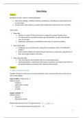
Data Mining
Chapter 1
Statistical learning = tools for understanding data
Supervised: building a statistical model for predicting or estimating an output based on one
or more inputs
Unsupervised: inputs without an output; learn relationships and structure from such data
Sorts of data
Wage data
o Examine a number of factors that relate to wages for a group of people (men)
o To understand the association between age and education, as well as the calander
year, on his wage
o Predicting a continuous or quantitative output value regression problem
Stock market data
o Predicting a non-numerical value; categorical or qualitative output classification
problem
o Goal is predict whether the index increase or decrease on a given day, using the past 5
days’ percentage changes in the index
Gene expression data
o Only observing the input variables with no corresponding output
o Clustering problem = understand which types of customers are similar to each other by
grouping individuals according to their observed characteristics
Chapter 2
2.1 What is statistical learning?
Example: the goal is to develop an accurate model that can be used to predict sales on the basis of
the 3 media budgets
Input variables = X ( X1, X2, X3 …)
Different names:
- Predictors
- Independent variable
- Features
- Variables
Output variables = Y
Different names:
- Response
- Dependent variable
Relationship between X and Y in his general form:
f : some fixed but unknown function of X 1, …, Xp
1
, o may involve more than one variable
ԑ : random error term
o independent of X
o has mean zero
Example:
Income is a simulated data set, so f is
known and is the blue curve in the right-
handed panel
The vertical lines represent the error
term ԑ some lie above the blue curve and
some under it.
Overall, the errors have +/- mean zero
2.1.1 Why estimating f?
There are 2 main reasons that we may wish to estimate f: (1) prediction and (2) inference
(1) Prediction
A set of inputs X are available, but the output Y is not easily obtained.
We predict the Y using
: the estimate for f treated as a black box (not concerned with the exact form of
, provided that it yield accurate predictions for Y)
: the resulting prediction for Y
o The accuracy depends on:
Reducible error = improve the accuracy of by using the most
appropriate statistical learning technique to estimate f
BUT there will still be some error in it
Irreducible error = Y is also a function of ԑ, which cannot be
predicted using X. no matter how well we estimate f, we cannot
reduce the error introduced by ԑ.
It is larger than zero because ԑ may contain unmeasured variables
that are useful in predicting Y. there are unmeasured, so f cannot use
them for its prediction.
Assume for a moment that both and X are fixed, the only variability comes from ԑ.
2
, : average or expected value of the squared difference between
predicted and actual value of Y
Var(ԑ) : variance associated with the error term ԑ
Focus of this book: minimize the reducible error
(2) Inference
Interested in the association between Y and X 1, …, Xp
Answering the following questions:
1. Which predictor are associated with the response?
2. What is the relationship between the response and each predictor?
3. Can the relationship between Y and each predictor be adequately summarized using a
linear equation, or is the relationship more complicated?
Some models can be conducted both for prediction and inference. (ex. Real estate setting: some are
interested in crime rate, some are interested in association between the price of a house and a view
of the river)
2.1.2 How to estimate f?
Training data = use the observations to train/teach our method how to estimate f.
It consists of
xij = value of the jth predictor/input for observation i (
)
Our goal is to apply a statistical learning method to the training data in order to estimate the
unknown function f. Or in other words , we want to find an such that .
(1) Parametric methods
Two steps:
1) Make an assumption about the functional form or shape of f .
Ex. Linear model:
Instead of having to estimate an entirely arbitrary p-dimensional function f(X), only
estimate p + 1 coefficients β0,β1, …, βp .
2) After a model has been selected, we need a procedure that uses training data to fit
or train the model
Ex. Linear model:
It reduces the problem of estimating f down to one of estimating a set of parameters.
Disadvantage: Choosing a model that not matches the true unknown form of f.
3
, Try to address this by choosing a more flexible model BUT requires estimating
more parameters.
These more complex models can lead to overfitting the data (they follow
errors too closely)
True function of f linear model fit by least squares
(2) Non-parametric methods
They seek an estimate of f that gets as close to the data points as possible without being too
rough or wiggly. You don’t choose a shape, so they have the potential to accurately fit a
wider range of possible shapes for f.
Disadvantage: they do not reduce the problem to a small number of parameters, a very large
number of observations is required in order to obtain an accurate estimate for f.
Ex. Thin-plate-spline: it does not impose any pre-specified model on f, attempts to procedure
an estimate for f that is close as possible to the observed data. The data analyst must select a
level of smoothness. BUT the spline fit is way more variable than the true function f.
( overfitting)
True function of f thin- plate spline fit
4