Macroeconomics 214
Chapter 5
A Closed-Economy One-Period Macro-Economic Model
Learning objectives
Define and construct a competitive equilibrium for the closed economy one period
macroeconomic (CEOP) model
Show that the competitive equilibrium and the Pareto optimum for the CEOP model
are the same thing
Analyse and interpret the effects of changes in exogenous variables in the CEOP
model
Decompose the effects of an increase in total factor productivity in the CEOP model
into income and substitution effects
Analyse the effects of distorting labor income tax in in the simplified CEOP model
Analyse the determinants of the size of government and private consumption
In this chapter, we take the microeconomic behaviour from chapter 4, build it into a one-
period model of the economy and then use that to study the effects of government spending
and changes in total factor productivity. This will help us build up some economic intuition
about how the economy works, which we ca develop further in later chapters. We will be
able to see how under certain assumptions, markets will be able to produce economic
outcomes that are social efficient. An outcome that is considered to be socially efficient is
one that is allocatively efficient. This implies that goods and services are produced in
quantities such that would make consumers happy in the allocation of said goods and
services.
Closed-Economy One-Period Model
There are 3 key agents in the one-period macro model: the representative consumer (whose
aim it is to optimise utility), the representative firm (whose aim it is to maximise profits) and
government. Government purchase goods (g) via tax revenue that it collects from
consumers (T). In the beginning, we assume that T is a lump-sum tax. All 3 of these
economic agents interact together in competitive markets where everyone is a price taker. In
a competitive equilibrium, this means that all markets clear. Prices are such tat quantity
supplies equals quantity demands in each market. The experiments tell us what the model
says about the economy, such as the effects of changes in government spending and in total
factor productivity.
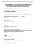
Figure 5.1: A model takes exogenous variables and determines endogenous variables
In this model,
government
expenditure and
taxation are given
exogenous
variables. These
, variables will be changed in order to shock the model, to see the effect it has on the
endogenous variables.
We assume the following in this chapter:
Government will deal with a budget constraint whereby government expenditure must
be equal to taxation – they will deal with a balanced budget – this assumption allows
us to understand fiscal policy. This particular budget constraint has important
implications in this model
Government cannot borrow money – there is not loan market.. This assumption is
dropped in chapter 9
Competitive Equilibrium
Both the representative consumer and the representative firm optimizes given relative
market prices. This means the supply equals demand and so markets will clear. This also
means that the labor market will clear. This is important because at this stage of the model,
we actually only have 1 price (real wage). This is the case because in this model we are
exchanging labor for goods. A competitive equilibrium is a set of endogenous quantities (in
this case, consumption, labor supply, labor demand, taxes and output) and an endogenous
real wage such that given the exogenous variables (government expenditure, total factor
productivity and capital) several aspects can be satisfied. The assumption that capital stock
is constant still applies. At a competitive equilibrium, the following will be satisfied:
The representative consumer will choose consumption and labor supply to make him/
herself as well off as possible given their budget constraint, the real wage, the level
of taxation and the dividend income.
The representative firm will choose the quantity of labor demanded to maximise
profits, with the maximised output being equal to our earlier stated production
function, and the maximised profits being the dividend equalled to output minus input
costs (the real market wage multiplied by the quantity of labour demanded).
The labor market will clear. The quantity of labor demanded will be equal to the
quantity of labour supplied.
The government’s budget constraint must be satisfied (g = T)
Income-Expenditure Identity
Once the competitive equilibrium is obtained, we find that the income-expenditure identity is
different to that of Chapter 4. Here, output is equal to the sum of consumption and
government expenditure. This is the case due to the assumptions we have made:
It is a closed economy therefore there are not net exports
Investments = 0. This is just to simplify the model.
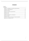
The production function
Chapter 5
A Closed-Economy One-Period Macro-Economic Model
Learning objectives
Define and construct a competitive equilibrium for the closed economy one period
macroeconomic (CEOP) model
Show that the competitive equilibrium and the Pareto optimum for the CEOP model
are the same thing
Analyse and interpret the effects of changes in exogenous variables in the CEOP
model
Decompose the effects of an increase in total factor productivity in the CEOP model
into income and substitution effects
Analyse the effects of distorting labor income tax in in the simplified CEOP model
Analyse the determinants of the size of government and private consumption
In this chapter, we take the microeconomic behaviour from chapter 4, build it into a one-
period model of the economy and then use that to study the effects of government spending
and changes in total factor productivity. This will help us build up some economic intuition
about how the economy works, which we ca develop further in later chapters. We will be
able to see how under certain assumptions, markets will be able to produce economic
outcomes that are social efficient. An outcome that is considered to be socially efficient is
one that is allocatively efficient. This implies that goods and services are produced in
quantities such that would make consumers happy in the allocation of said goods and
services.
Closed-Economy One-Period Model
There are 3 key agents in the one-period macro model: the representative consumer (whose
aim it is to optimise utility), the representative firm (whose aim it is to maximise profits) and
government. Government purchase goods (g) via tax revenue that it collects from
consumers (T). In the beginning, we assume that T is a lump-sum tax. All 3 of these
economic agents interact together in competitive markets where everyone is a price taker. In
a competitive equilibrium, this means that all markets clear. Prices are such tat quantity
supplies equals quantity demands in each market. The experiments tell us what the model
says about the economy, such as the effects of changes in government spending and in total
factor productivity.
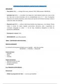
Figure 5.1: A model takes exogenous variables and determines endogenous variables
In this model,
government
expenditure and
taxation are given
exogenous
variables. These
, variables will be changed in order to shock the model, to see the effect it has on the
endogenous variables.
We assume the following in this chapter:
Government will deal with a budget constraint whereby government expenditure must
be equal to taxation – they will deal with a balanced budget – this assumption allows
us to understand fiscal policy. This particular budget constraint has important
implications in this model
Government cannot borrow money – there is not loan market.. This assumption is
dropped in chapter 9
Competitive Equilibrium
Both the representative consumer and the representative firm optimizes given relative
market prices. This means the supply equals demand and so markets will clear. This also
means that the labor market will clear. This is important because at this stage of the model,
we actually only have 1 price (real wage). This is the case because in this model we are
exchanging labor for goods. A competitive equilibrium is a set of endogenous quantities (in
this case, consumption, labor supply, labor demand, taxes and output) and an endogenous
real wage such that given the exogenous variables (government expenditure, total factor
productivity and capital) several aspects can be satisfied. The assumption that capital stock
is constant still applies. At a competitive equilibrium, the following will be satisfied:
The representative consumer will choose consumption and labor supply to make him/
herself as well off as possible given their budget constraint, the real wage, the level
of taxation and the dividend income.
The representative firm will choose the quantity of labor demanded to maximise
profits, with the maximised output being equal to our earlier stated production
function, and the maximised profits being the dividend equalled to output minus input
costs (the real market wage multiplied by the quantity of labour demanded).
The labor market will clear. The quantity of labor demanded will be equal to the
quantity of labour supplied.
The government’s budget constraint must be satisfied (g = T)
Income-Expenditure Identity
Once the competitive equilibrium is obtained, we find that the income-expenditure identity is
different to that of Chapter 4. Here, output is equal to the sum of consumption and
government expenditure. This is the case due to the assumptions we have made:
It is a closed economy therefore there are not net exports
Investments = 0. This is just to simplify the model.
The production function