Chapter 3 Basic Analysis of Resistive Circuits
3.1 Number of Independent Circuit Equations
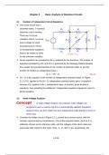
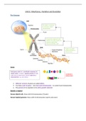
The circuit shown has 4
essential nodes, 7 essential R1 R4
a c
branches, and 4 meshes.
There are 14 circuit
R5 R8
variables, that is, a current V + R3 R6
SRC _
and a voltage for each
essential branch. Hence,
14 simultaneous equations
R2 b R7 d
have to be written to solve Figure 3.1.1
for the unknown variables.
Seven equations are provided by the v-i relations for the branches. The number of
equations provided by KCL and KVL is governed by the following relation between
the number of essential branches B, the number of essential nodes N, and the
number of meshes or independent loops L:
B = L + (N – 1) (3.1.1)
(N – 1) in this equation is the number of independent essential nodes. In Figure
3.1.1, KCL applied to the (N – 1) independent essential nodes gives 3 equations
whereas KVL applied to the L independent loops, or meshes, gives another 4
equations, thus providing the additional 7 independent equation required to solve for
all the variables.
3.2 Node-Voltage Analysis
Concept In node-voltage analysis, the unknown node voltages are
assigned in such a manner that KVL is automatically satisfied. Equations
based on KCL are then written for each independent node directly in terms of
Ohm’s law.
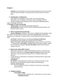
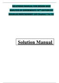
Consider the bridge circuit of Figure 3.2.1, excited by a current source, with the
resistors represented by conductances. One of the essential nodes, such as d, is
arbitrarily chosen as the reference node, and the voltages of the other nodes are
expressed with respect to this node. Thus, Va, Vb, and Vc are, respectively, the
3-1/16
, voltage drops from nodes a, b, and c to d.
The assignment
a Va
of node
voltages in this a
+ +
manner Vab Vac
automatically – –
G1 G2
satisfies KVL. – Vcb +
Vb Vc
To verify this, ISRC Gsrc
b c
consider a G5
mesh such as G4 G3
+
acb and +
Vbd Vcd
express the – –
voltage drops
d
across the d
Figure 3.2.1
circuit elements
in this mesh in terms of the assigned node voltages:
Vac = Va – Vc
Vcb = Vc – Vb
Vab = Va – Vb, or –Vab = –Va + Vb
When these equations are added, the node voltages on the RHS cancel out,
giving: Vac + Vcb – Vab = 0, which is KVL for mesh acb. The same is true of any other
mesh or loop in the circuit.
The next step is to write KCL for each of the nodes a, b, and c. Considering node a,
the total current leaving this node through G1, G2, and Gsrc is: G2(Va – Vc) + G1(Va –
Vb) + GsrcVa. This current must equal the source current ISRC entering the node.
Combining the coefficients of Va, Vb, and Vc gives for KCL at node a:
(Gsrc + G1 + G2)Va –G1Vb –G2Vc = ISRC (3.2.1)
As for nodes b and c, there is no source current entering these nodes. The current
leaving node b through the conductances connected to this node is: G1(Vb – Va) +
G5(Vb – Vc) + G4Vb. Combining coefficients of the variables, gives for KCL at node b:
–G1Va +(G1 + G4 + G5)Vb –G5Vc =0 (3.2.2)
The current leaving node c through the conductances is: G2(Vc – Va) + G5(Vc – Vb) +
G3Vc. Combining coefficients of the variables, gives for KCL at node c.
3-2/16
, –G2Va –G5Vb +(G2 + G3 +G5)Vc =0 (3.2.3)
Comparing Equations 3.2.1 to 3.2.3, a definite pattern emerges for writing the node-
voltage equation for any node n, which may be summarized as follows:
Procedure
1. The voltage of node n is multiplied by the sum of all the conductances connected
directly to this node. This sum is the self-conductance of node n.
2. The voltage of every other node is multiplied by the conductance connected directly
between node n and the given node. This is the mutual conductance between the
two nodes. If there is no such conductance, the coefficient is zero. The sign of a
nonzero coefficient is always negative, because the current flowing away from node
n toward the given node is proportional to the voltage of node n minus that of the
given node.
3. The LHS of the node-voltage equation for node n is the sum of the terms from the
preceding steps, ordered as the unknown node voltages. This sum is the total
current leaving node n through the conductances connected to this node.
4. The RHS of the equation is equal to any source current entering node n.
Ideal resistors are bilateral, that is, the resistance is the same for both directions of
current. This means that the mutual conductance terms in the equations of any two
given nodes are the same. For example, the current flowing from node b toward
node c is G5(Vb – Vc) in Figure 3.2.1, whereas the current flowing from node c toward
node b is G5(Vc – Vb). The coefficient of Vc in the node-voltage equation for node b,
which is –G5 in Equation 3.7.2, is the same as the coefficient of Vb in the node-
voltage equation for node c (Equation 3.7.3). When ordered in a matrix, or array, the
conductance coefficients are symmetrical with respect to the diagonal, in the
absence of dependent sources. This is a useful check on the node-voltage
equations.
3-3/16
3.1 Number of Independent Circuit Equations
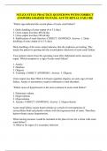
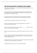
The circuit shown has 4
essential nodes, 7 essential R1 R4
a c
branches, and 4 meshes.
There are 14 circuit
R5 R8
variables, that is, a current V + R3 R6
SRC _
and a voltage for each
essential branch. Hence,
14 simultaneous equations
R2 b R7 d
have to be written to solve Figure 3.1.1
for the unknown variables.
Seven equations are provided by the v-i relations for the branches. The number of
equations provided by KCL and KVL is governed by the following relation between
the number of essential branches B, the number of essential nodes N, and the
number of meshes or independent loops L:
B = L + (N – 1) (3.1.1)
(N – 1) in this equation is the number of independent essential nodes. In Figure
3.1.1, KCL applied to the (N – 1) independent essential nodes gives 3 equations
whereas KVL applied to the L independent loops, or meshes, gives another 4
equations, thus providing the additional 7 independent equation required to solve for
all the variables.
3.2 Node-Voltage Analysis
Concept In node-voltage analysis, the unknown node voltages are
assigned in such a manner that KVL is automatically satisfied. Equations
based on KCL are then written for each independent node directly in terms of
Ohm’s law.
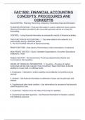
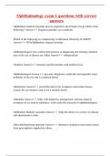
Consider the bridge circuit of Figure 3.2.1, excited by a current source, with the
resistors represented by conductances. One of the essential nodes, such as d, is
arbitrarily chosen as the reference node, and the voltages of the other nodes are
expressed with respect to this node. Thus, Va, Vb, and Vc are, respectively, the
3-1/16
, voltage drops from nodes a, b, and c to d.
The assignment
a Va
of node
voltages in this a
+ +
manner Vab Vac
automatically – –
G1 G2
satisfies KVL. – Vcb +
Vb Vc
To verify this, ISRC Gsrc
b c
consider a G5
mesh such as G4 G3
+
acb and +
Vbd Vcd
express the – –
voltage drops
d
across the d
Figure 3.2.1
circuit elements
in this mesh in terms of the assigned node voltages:
Vac = Va – Vc
Vcb = Vc – Vb
Vab = Va – Vb, or –Vab = –Va + Vb
When these equations are added, the node voltages on the RHS cancel out,
giving: Vac + Vcb – Vab = 0, which is KVL for mesh acb. The same is true of any other
mesh or loop in the circuit.
The next step is to write KCL for each of the nodes a, b, and c. Considering node a,
the total current leaving this node through G1, G2, and Gsrc is: G2(Va – Vc) + G1(Va –
Vb) + GsrcVa. This current must equal the source current ISRC entering the node.
Combining the coefficients of Va, Vb, and Vc gives for KCL at node a:
(Gsrc + G1 + G2)Va –G1Vb –G2Vc = ISRC (3.2.1)
As for nodes b and c, there is no source current entering these nodes. The current
leaving node b through the conductances connected to this node is: G1(Vb – Va) +
G5(Vb – Vc) + G4Vb. Combining coefficients of the variables, gives for KCL at node b:
–G1Va +(G1 + G4 + G5)Vb –G5Vc =0 (3.2.2)
The current leaving node c through the conductances is: G2(Vc – Va) + G5(Vc – Vb) +
G3Vc. Combining coefficients of the variables, gives for KCL at node c.
3-2/16
, –G2Va –G5Vb +(G2 + G3 +G5)Vc =0 (3.2.3)
Comparing Equations 3.2.1 to 3.2.3, a definite pattern emerges for writing the node-
voltage equation for any node n, which may be summarized as follows:
Procedure
1. The voltage of node n is multiplied by the sum of all the conductances connected
directly to this node. This sum is the self-conductance of node n.
2. The voltage of every other node is multiplied by the conductance connected directly
between node n and the given node. This is the mutual conductance between the
two nodes. If there is no such conductance, the coefficient is zero. The sign of a
nonzero coefficient is always negative, because the current flowing away from node
n toward the given node is proportional to the voltage of node n minus that of the
given node.
3. The LHS of the node-voltage equation for node n is the sum of the terms from the
preceding steps, ordered as the unknown node voltages. This sum is the total
current leaving node n through the conductances connected to this node.
4. The RHS of the equation is equal to any source current entering node n.
Ideal resistors are bilateral, that is, the resistance is the same for both directions of
current. This means that the mutual conductance terms in the equations of any two
given nodes are the same. For example, the current flowing from node b toward
node c is G5(Vb – Vc) in Figure 3.2.1, whereas the current flowing from node c toward
node b is G5(Vc – Vb). The coefficient of Vc in the node-voltage equation for node b,
which is –G5 in Equation 3.7.2, is the same as the coefficient of Vb in the node-
voltage equation for node c (Equation 3.7.3). When ordered in a matrix, or array, the
conductance coefficients are symmetrical with respect to the diagonal, in the
absence of dependent sources. This is a useful check on the node-voltage
equations.
3-3/16