Aantekeningen colleges ICT
Mathematical fundamentals (ma 2-9)
Parameter = constant & make calculations more general, usually considered positive
Operations + - / *
Opening parentheses:
Introducing parentheses (= factoring):
Parameter equation solving: | Factoring: | Solving quadratic equations:(check afterwards!)
| |
| |
| |
Multiple variables: solve how one variable depends on the other choose simplest option
Substitution approach ----------------------->
Elimination approach
------------------------------------------->
Function = formula describing how one quantity depends on other quantities (y = f(x) -> f(x) = x^2 )
x = independent variable y = dependent variable
Functions have a domain (x) = set of all possible input values & range (y) = set of all possible output values
[ of ] = tot die waarde < of > = bij infinity
Limit (L): L is the limit of the function f(x) when f(x) approaches L in case x approaches a lim
x→ ∞
f ( x ) =L
Only defined when approached from either side is the same: lim
x ↑a
f ( x )=lim f ( x )=L
x ↓a
Limits can be found by filling out x = a in f(x)
Exceptions: limits at infinity and infinite ‘limits’ (vb. f(x) = b + 1 / x)
g (x)
Limits for rational functions (vb. f ( x )= )
h( x)'
Divide by highest power in denominator
Result depends on highest powers in nominator and denominator
Highest power numerator = denominator limit = constant
Highest power numerator < denominator limit = 0
Highest power numerator > denominator no limit (± ∞ )
Local slope (derivative) differentiation = calculating deriv of a function
- ( f +g )' ( x )=f ' ( x ) + g' ( x )
- ( f −g )' ( x ) =f ' ( x )−g' ( x )
- ( Cf )' ( x )=C f ' ( x )
- Product rule: h ( x )=f ( x ) g ( x ) → h' ( x )=f ' ( x ) g ( x ) + f ( x ) g ' ( x )
- Chain rule: h ( x )=f ( g ( x ) ) =f ∙ g ( x ) →h' ( x )=f ' ( g ( x ) ) g '( x)
f (x ) g ( x ) f ' ( x ) −f ( x ) g ' (x)
- Quotient rule: h ( x )= → h' ( x )= 2
g ( x) (g ( x ))
Shapes of common functions:
o Parabolic (no asymp)
o Cubic (no asymp)
o Square root func
o Hyperbolic func
o Exponential growth(e a) / decay (e−a)
Plan to draw graphs:
I. Intersection points x-axis solve y = f (x) = 0
II. Intersection points y-axis fill in x = 0 in y = f (x)
III. lim f ( x )
Horizontal asymptotes find limit x→ ±∞
p (x)
IV. Vertical asymptotes for rational functions x values for which q (x) = 0 ?
q( x )
V. X values of maxima / minima solve f ‘ (x) = 0
VI. Y values at maxima / minima fill in x value(s) in f (x)
VII. Sketch all possible graphs
, Introduction to modeling (di 3-9)
Model = simplified abstraction of reality focus on only certain aspects of study object
Types of models: Animal/disease Conceptual/verbal Cartoon Quantitative
Why quantitative models: increased precision/remove uncertainty | predicition (inter- & extrapolation) | possibility to
analyze (simulation, mathematics) | automated analysis | explain ‘complex’ system behaviour based on individual
components | integrative view on data acquired at different levels
Models based on observations cannot be proven correct (only in mathematical statements)
Model falsification: bewijs waarom model incorrect is
Model validation: verify predictions by experimentation increase confidence in model
Scope of model (beschrijft bepaald deel / specific circumstances)
Mechanistic models describe mechanism underlying observed behaviour understanding
Descriptive/phenomenological models summarize data powerful for prediction
Damped oscillations vs. persistent oscillations -------------------------------------------------------->
Negative feedback can lead to oscillations
Modeling of pathway include isoforms in model compare model & experiment knockout of isoforms result
Differential equations I (di 3-9)
Cartoon network models:
Based on verbal description | nodes: molecular species | arrows: molecular interactions (form, degr, regulation)
Mathematical network models:
Remove uncertainty of model behaviour by becoming quantitive
Modeling: Ordinary Differential Equations (ODEs) describe dynamics | arrows = quantitative eaction rates
(State) variables: abundance of modeled molecular species | can vary over time
Parameters: values are fixed over studied time scale | characterizes environmental effects & interactions (vb. degr rate)
In biology, parameters are positive
Reaction rates: predict changes over time
- Depends on: conc of reactants | environmental conditions (temp, pH)
If rate is known, reactions can be described as Ordinary Differential Equations (ODEs)
ODE assumptions: reaction rates are approximated:
I. Well-mixed environment rates considered independent of position in space (but: spacial structure in cells)
II. Many molecules are present continuous rather than discrete (but: some processes rely on only 1e 5 molecs)
Translation from cartoon network to a quantitative description (here: reactions)
------------------>
Law of mass-action: reaction rate is proportional to the product of the concs of the reactants
k, k1, k2, k3 = rate constants
k 0 A k1 da(t )
=rate of change of [ A ] =k 0−k 1 a ( t )=rate of production−rate of decay
→ → dt
Cartoon to quantitative description: chemical reaction network reaction rates assumptions ODE
Differential equations II (wo 4-9)
Analysis of ODEs: I. Analytical/symbolic solution II. Numerical simulationIII. Model analysis
Ak da
Analytical: =−ka a ( t )=D e−kt = exponential decay (D = initial conc)
→ dt
Numerical: in silico experi how does system behave?
Predict system behaviour over time for given conditions | use numerical simulations in software packages (vb. R)
da(t ) a ( t+ h )−a (t)
Approximation of solution: Euler’s method =f (a (t ) ) f ( a (t)) ≈ a ( t +h ) ≈ a ( t )+ hf ¿ )
dt h