Lecture notes Bayesian Statistics
Lecture 1: Introduction & preliminaries
The core of Bayes
- (Re-)allocating credibility in light of observations
- Credibility = probability
Inference
- Inference: what is true about the world, given what we see?
- Our inferences make sense only if our assumptions hold.
Reallocating probability
- Two ways of collecting evidence
o Evidence can be in favour or against some hypothesis; both work in the Bayesian
framework
o You can eliminate the impossible or implicate a possible outcome
- Noisy data and probabilistic inference
o Unfortunately, every measurement is noisy
o We collect only finite data, and many factors make each sample unique
Three goals of statistical inference:
- Parameter estimation
o What is parameter θ, given data D?
- Prediction of new observations
o What will xˆ ̸∈ D be, given parameters θ (learned using D)?
- Model comparison
o There are multiple ways we can construct P(θ | D)? Which one is the ‘best’?
Probabilistic inference:
- Inference is reallocating probability so that it fits the data and assumptions optimally.
- Consistent possibilities become more credible, inconsistent ones become less credible.
- Uncertainty is captured in probability distributions (instead of point estimates).
Model
- A model is a set of hypotheses about the process that created the data
- Model parameters are the control buttons and dials of the model; different parameter
settings generate data with different properties
- Desiderata (not strict!)
o We must be able to write down the model math
o The parameters of the model should have clear meaning
o Ideally: the predictions of the model are similar to the actual observed distribution of
the data
- Model fit does not equal truth!
Steps of Bayesian analysis
1. Identify relevant variables for the study
, 2. Define a descriptive, mathematical model of the data, given the parameters
3. Specify the prior allocation of credibility (before observing data)
4. Use Bayesian inference to re-allocate probabilities across parameter values, given the
observed data and the prior beliefs
5. Verify that the posterior matches the data (reasonably well)
Frequentist definition of probability: relative frequency (3/6)
Bayesian definition of probability: probability as degree of belief
The three rules of probabilities:
- A probability is non-negative (but can be zero)
- The sum of all probabilities over all the sample space (=outcomes) must be one
- For any two mutually exclusive events, the probability that either occurs is the sum of the
probabilities of the individual events
If the sample space is discrete, each outcome has its own probability, also known as its probability
mass. The total area under the curve probability density function p(x) integrates (≈ continuous sum)
to one.
- Mean: E [ x ] =∑ P ( x ) x
x
Variance: Var [ x ]=∑ P ( x ) ( x−E [ x ] )
2
-
x
- Highest density interval (HDI) = confidence interval
- Joint probability: P ( x , y )=P ( y , x )
P(x , y)
- Conditional probability: P ( x| y )=
P( y )
- Marginal probability: P ( x )=∑ P(x , y )
y
- Independence: P ( x , y )=P ( x ) P( y)
P ( y∨x) P( x ) P( y∨x) P( x)
Bayes’ rule: P ( x| y )= =
- P ( y) ∑ P( y ∨x' )P(x ' )
x'
o Allows us to infer about things we do not directly observe
o Posterior: P ( x| y )
o Likelihood: P( y ∨x)
o Prior: P( x )
o Evidence: P( y )
Bayesian updating:
- We start with a prior and obtain the posterior.
- This posterior becomes the prior for the next observation!
- If we iterate this, we end up with a distribution in which the prior has (almost) no effect: the
idea of Bayesian updating.
To read: Probability theory recap: Kruschke, chapters 2, 4, 5.1 and 5.2.
Lecture 2: Bayesian inference
Bernoulli likelihood
, - We construct a model of flipping a coin, relating the outcome with some parameter θ:
- We define p(y = 1 | θ) = θ (with θ ∈ [0, 1])
- Given this, we want to know the posterior p(θ | y1, y2, . . . , yN )
- For Bayesian inference we need the likelihood function p(y | θ):
o p(y = 1 | θ) = θ and p(y = 0 | θ) = 1 − θ
o Bernoulli: p ( y|θ )=θ y ( 1−θ )1− y
- For Bayesian inference we need a prior distribution on the parameter θ.
- Observing data determines the likelihood of θ.
- The posterior is obtained by multiplying for each possible θ the likelihood and the prior, and
normalizing by p ( D )=∑ p ( D|θ ) p(θ )
' '
θ'
Practical problems with Bayesian inference
- The difficulty is often in the normalizing integral p ( D )=∫ p ( D|θ ) p ( θ ) dθ
o An integral can be difficult to solve, m-dimensional ones can rarely be solved
analytically
- Approximate techniques exist (next week!), but they require (much) more computation time
Convenient prior distribution
- If we can compute the model evidence analytically, inference becomes that much easier
- If the prior and the posterior have the same form, we could keep updating (= observing more
data), but remain in the same model
- If prior and likelihood combine to a posterior with the same form as the prior, the prior is
called conjugate
a−1
θ ( 1−θ )b−1
- The beta distribution fits the bill: p ( θ|a , b )=beta ( θ|a , b )=
B (a , b)
- Proof:
Beta distribution
θ a−1 ( 1−θ )b−1
- p ( θ|a , b )=beta ( θ|a , b )=
B (a , b)
, - The normalizing constant is the beta function:
1
Γ (a) Γ (b) ( a−1 ) ! ( b−1 ) !
B ( a , b )=∫ θ
a−1
( 1−θ )b−1 dθ= =
0 Γ (a+b) ( a+b−1 ) !
- If the prior has form X, and it is conjugate to the likelihood, then the posterior also has form X
- Starting with a beta prior and conjugate likelihood (Bernoulli); no matter how much more
observations come in, the distribution remains a beta
o This allows us to repeat the procedure ad infinitum
- The beta prior is conjugate to the Bernoulli likelihood, so the posterior is again a beta
distribution
- Its parameters are sometimes called pseudo observations; they reflect ‘fake’ observations for
either heads or tails. The total a + b is the number of prior observations
- Pseudo observations a and b specify unseen data
- The expectation of the beta distribution is µ = a/(a + b) and the variance is µ(1−µ) / 1+a+b
- The beta prior is convenient for parameters θ ∈ [0, 1], but many other distributions over this
domain exist and are valid choices
- With a beta prior and Bernoulli likelihood (a conjugate pair), we immediately know the
posterior is a beta distribution as well:
o a ' =a+ z
o b ' =b+ N− z
Posterior compromises prior and likelihood
- The mode of a distribution:
o Take the derivative of the logarithm of PDF
o Find the parameters for which the derivative is zero
- In the modes of the distributions
o Maximum likelihood estimate (MLE):
z
θ MLE =
N
o Mode of prior:
a−1
θ Prior=
a+ b−2
o Maximum a posteriori (MAP):
a+ z−1
θ MAP=
a+b + N−2
o In the expectations of the distributions
1
Expectation: E [ θ ] =∫ θp ( θ ) dθ
0
a
Prior: E [ θ ] =
a+b
a+ z
Posterior: E [ θ∨D ] =
a+b+ N
Predicting the value for a new observation x∗ has huge application potential. We need predictive
distributions. We have (unwillingly) already seen the prior predictive distribution:
p ( x )=∫ p ( x |θ ) p ( θ ) dθ .
¿ ¿
See how similar this is to the marginal likelihood! However, we compute the marginal likelihood for
Lecture 1: Introduction & preliminaries
The core of Bayes
- (Re-)allocating credibility in light of observations
- Credibility = probability
Inference
- Inference: what is true about the world, given what we see?
- Our inferences make sense only if our assumptions hold.
Reallocating probability
- Two ways of collecting evidence
o Evidence can be in favour or against some hypothesis; both work in the Bayesian
framework
o You can eliminate the impossible or implicate a possible outcome
- Noisy data and probabilistic inference
o Unfortunately, every measurement is noisy
o We collect only finite data, and many factors make each sample unique
Three goals of statistical inference:
- Parameter estimation
o What is parameter θ, given data D?
- Prediction of new observations
o What will xˆ ̸∈ D be, given parameters θ (learned using D)?
- Model comparison
o There are multiple ways we can construct P(θ | D)? Which one is the ‘best’?
Probabilistic inference:
- Inference is reallocating probability so that it fits the data and assumptions optimally.
- Consistent possibilities become more credible, inconsistent ones become less credible.
- Uncertainty is captured in probability distributions (instead of point estimates).
Model
- A model is a set of hypotheses about the process that created the data
- Model parameters are the control buttons and dials of the model; different parameter
settings generate data with different properties
- Desiderata (not strict!)
o We must be able to write down the model math
o The parameters of the model should have clear meaning
o Ideally: the predictions of the model are similar to the actual observed distribution of
the data
- Model fit does not equal truth!
Steps of Bayesian analysis
1. Identify relevant variables for the study
, 2. Define a descriptive, mathematical model of the data, given the parameters
3. Specify the prior allocation of credibility (before observing data)
4. Use Bayesian inference to re-allocate probabilities across parameter values, given the
observed data and the prior beliefs
5. Verify that the posterior matches the data (reasonably well)
Frequentist definition of probability: relative frequency (3/6)
Bayesian definition of probability: probability as degree of belief
The three rules of probabilities:
- A probability is non-negative (but can be zero)
- The sum of all probabilities over all the sample space (=outcomes) must be one
- For any two mutually exclusive events, the probability that either occurs is the sum of the
probabilities of the individual events
If the sample space is discrete, each outcome has its own probability, also known as its probability
mass. The total area under the curve probability density function p(x) integrates (≈ continuous sum)
to one.
- Mean: E [ x ] =∑ P ( x ) x
x
Variance: Var [ x ]=∑ P ( x ) ( x−E [ x ] )
2
-
x
- Highest density interval (HDI) = confidence interval
- Joint probability: P ( x , y )=P ( y , x )
P(x , y)
- Conditional probability: P ( x| y )=
P( y )
- Marginal probability: P ( x )=∑ P(x , y )
y
- Independence: P ( x , y )=P ( x ) P( y)
P ( y∨x) P( x ) P( y∨x) P( x)
Bayes’ rule: P ( x| y )= =
- P ( y) ∑ P( y ∨x' )P(x ' )
x'
o Allows us to infer about things we do not directly observe
o Posterior: P ( x| y )
o Likelihood: P( y ∨x)
o Prior: P( x )
o Evidence: P( y )
Bayesian updating:
- We start with a prior and obtain the posterior.
- This posterior becomes the prior for the next observation!
- If we iterate this, we end up with a distribution in which the prior has (almost) no effect: the
idea of Bayesian updating.
To read: Probability theory recap: Kruschke, chapters 2, 4, 5.1 and 5.2.
Lecture 2: Bayesian inference
Bernoulli likelihood
, - We construct a model of flipping a coin, relating the outcome with some parameter θ:
- We define p(y = 1 | θ) = θ (with θ ∈ [0, 1])
- Given this, we want to know the posterior p(θ | y1, y2, . . . , yN )
- For Bayesian inference we need the likelihood function p(y | θ):
o p(y = 1 | θ) = θ and p(y = 0 | θ) = 1 − θ
o Bernoulli: p ( y|θ )=θ y ( 1−θ )1− y
- For Bayesian inference we need a prior distribution on the parameter θ.
- Observing data determines the likelihood of θ.
- The posterior is obtained by multiplying for each possible θ the likelihood and the prior, and
normalizing by p ( D )=∑ p ( D|θ ) p(θ )
' '
θ'
Practical problems with Bayesian inference
- The difficulty is often in the normalizing integral p ( D )=∫ p ( D|θ ) p ( θ ) dθ
o An integral can be difficult to solve, m-dimensional ones can rarely be solved
analytically
- Approximate techniques exist (next week!), but they require (much) more computation time
Convenient prior distribution
- If we can compute the model evidence analytically, inference becomes that much easier
- If the prior and the posterior have the same form, we could keep updating (= observing more
data), but remain in the same model
- If prior and likelihood combine to a posterior with the same form as the prior, the prior is
called conjugate
a−1
θ ( 1−θ )b−1
- The beta distribution fits the bill: p ( θ|a , b )=beta ( θ|a , b )=
B (a , b)
- Proof:
Beta distribution
θ a−1 ( 1−θ )b−1
- p ( θ|a , b )=beta ( θ|a , b )=
B (a , b)
, - The normalizing constant is the beta function:
1
Γ (a) Γ (b) ( a−1 ) ! ( b−1 ) !
B ( a , b )=∫ θ
a−1
( 1−θ )b−1 dθ= =
0 Γ (a+b) ( a+b−1 ) !
- If the prior has form X, and it is conjugate to the likelihood, then the posterior also has form X
- Starting with a beta prior and conjugate likelihood (Bernoulli); no matter how much more
observations come in, the distribution remains a beta
o This allows us to repeat the procedure ad infinitum
- The beta prior is conjugate to the Bernoulli likelihood, so the posterior is again a beta
distribution
- Its parameters are sometimes called pseudo observations; they reflect ‘fake’ observations for
either heads or tails. The total a + b is the number of prior observations
- Pseudo observations a and b specify unseen data
- The expectation of the beta distribution is µ = a/(a + b) and the variance is µ(1−µ) / 1+a+b
- The beta prior is convenient for parameters θ ∈ [0, 1], but many other distributions over this
domain exist and are valid choices
- With a beta prior and Bernoulli likelihood (a conjugate pair), we immediately know the
posterior is a beta distribution as well:
o a ' =a+ z
o b ' =b+ N− z
Posterior compromises prior and likelihood
- The mode of a distribution:
o Take the derivative of the logarithm of PDF
o Find the parameters for which the derivative is zero
- In the modes of the distributions
o Maximum likelihood estimate (MLE):
z
θ MLE =
N
o Mode of prior:
a−1
θ Prior=
a+ b−2
o Maximum a posteriori (MAP):
a+ z−1
θ MAP=
a+b + N−2
o In the expectations of the distributions
1
Expectation: E [ θ ] =∫ θp ( θ ) dθ
0
a
Prior: E [ θ ] =
a+b
a+ z
Posterior: E [ θ∨D ] =
a+b+ N
Predicting the value for a new observation x∗ has huge application potential. We need predictive
distributions. We have (unwillingly) already seen the prior predictive distribution:
p ( x )=∫ p ( x |θ ) p ( θ ) dθ .
¿ ¿
See how similar this is to the marginal likelihood! However, we compute the marginal likelihood for