Data Science
, Model evaluation
3
After having a trained model one would like to know the prediction capabilities on new, unseen, data
Model selection: comparing performance of different models, to identify best one
e
Model assessment: having chosen a final model, estimating how well it predicts on new data
&
Linear models for regression
S
example model troughout the course
Y =
A(X ,
B) +
- N(0 ga)
,
M
FoBmhm(X)
~
A(X ,
B) :
↳
Basic function/derived future
&
ex. In linear regression hm(X) =
Xm
Determine the model parameters using maximum likelihood
&
Take product/likelihood function
[(B 02) : re ,
2
Take logaritme
In 2(B 02) Nh(8)-(2)-(yn,
: -
-
Sh(xn))
3
Take derivatives
O
with respect to B e
with respect to 8
↳
In[(B 02) : (yn- Sh(xn))hm(xn) ,
=
0 so In 2(B :),
:
↓
: (Xx)"xy 02 : Z (yn-BXn)
Y
Generalization error
To determine the performance of a model, we define a loss function that measures the size of a prediction error
examples of loss functions
We want the error to be as small as possible as this
S
(Y E(x)))
squared error -
means that there is a high generalization
L(Y , (x)) Y E(X)
absolute error
=
-
Estimating the generalization error is often not possible,
3 types of errors
3
therefore we use estimate of prediction error
1 Err : E L(Y ,
E(x)) Err :
Er Err
2 Erro :
E[L(Y , (X)) It
, 3 er
: (yn , (xn))
Bias-variance decomposition
Err(xo) : EL/Y-E(X))"(X =
xo
=
(E[E(xo)] f(xo))2 E[(xo)
- + ·
ETE(xo)" -8 When we increase the polynomial,
=
Bias
&
((xo)) + Var((xo)) + 8
higher variance but lower bias
=
Bias + Varianee + G When decrease in polynomial,
&
variance of error lower variance but higher bias
S
variance of estimated model
&
squared bias of estimated model * We need to make a trade-off such
that the variance + bias are minimal
s
High variance, low bias Low variance, high bias
Data
When dealing with a data set, it is not possible to simulate additional data points to compute the
generalization errors and expected prediction error. We therefore need alternative procedures to estimate
the generalization and prediction errors. In the next three sections we will describe several of those
procedures 2
1
O
Data-rich situations: many data available
In-sample errors: calculating
errors from data on which
Training set Validation set Test set the model was trained
D Out-of-sample errors:
Used to test the model calculation errors from data
& that was excluded from the
Used to measure the performance training set
&
Used to train the data
⑨
Insufficient data: not enough data available
2
Information theoretical measures
&
The maximum log-likelihood is a measure for how well the model can describe the data, however we need
an penalty term that takes model complexity in account
3 Choose model with smallest AIC/BIC
-
Ale : - 2h([) + 2 (M 1) +
- Ble =
-2ln() + In (N) (M 1) +
, Model evaluation
3
After having a trained model one would like to know the prediction capabilities on new, unseen, data
Model selection: comparing performance of different models, to identify best one
e
Model assessment: having chosen a final model, estimating how well it predicts on new data
&
Linear models for regression
S
example model troughout the course
Y =
A(X ,
B) +
- N(0 ga)
,
M
FoBmhm(X)
~
A(X ,
B) :
↳
Basic function/derived future
&
ex. In linear regression hm(X) =
Xm
Determine the model parameters using maximum likelihood
&
Take product/likelihood function
[(B 02) : re ,
2
Take logaritme
In 2(B 02) Nh(8)-(2)-(yn,
: -
-
Sh(xn))
3
Take derivatives
O
with respect to B e
with respect to 8
↳
In[(B 02) : (yn- Sh(xn))hm(xn) ,
=
0 so In 2(B :),
:
↓
: (Xx)"xy 02 : Z (yn-BXn)
Y
Generalization error
To determine the performance of a model, we define a loss function that measures the size of a prediction error
examples of loss functions
We want the error to be as small as possible as this
S
(Y E(x)))
squared error -
means that there is a high generalization
L(Y , (x)) Y E(X)
absolute error
=
-
Estimating the generalization error is often not possible,
3 types of errors
3
therefore we use estimate of prediction error
1 Err : E L(Y ,
E(x)) Err :
Er Err
2 Erro :
E[L(Y , (X)) It
, 3 er
: (yn , (xn))
Bias-variance decomposition
Err(xo) : EL/Y-E(X))"(X =
xo
=
(E[E(xo)] f(xo))2 E[(xo)
- + ·
ETE(xo)" -8 When we increase the polynomial,
=
Bias
&
((xo)) + Var((xo)) + 8
higher variance but lower bias
=
Bias + Varianee + G When decrease in polynomial,
&
variance of error lower variance but higher bias
S
variance of estimated model
&
squared bias of estimated model * We need to make a trade-off such
that the variance + bias are minimal
s
High variance, low bias Low variance, high bias
Data
When dealing with a data set, it is not possible to simulate additional data points to compute the
generalization errors and expected prediction error. We therefore need alternative procedures to estimate
the generalization and prediction errors. In the next three sections we will describe several of those
procedures 2
1
O
Data-rich situations: many data available
In-sample errors: calculating
errors from data on which
Training set Validation set Test set the model was trained
D Out-of-sample errors:
Used to test the model calculation errors from data
& that was excluded from the
Used to measure the performance training set
&
Used to train the data
⑨
Insufficient data: not enough data available
2
Information theoretical measures
&
The maximum log-likelihood is a measure for how well the model can describe the data, however we need
an penalty term that takes model complexity in account
3 Choose model with smallest AIC/BIC
-
Ale : - 2h([) + 2 (M 1) +
- Ble =
-2ln() + In (N) (M 1) +