ML is learning from examples, which we will use to generalize over new data. 1) How to evaluate? Prec -> Sprvzd learning for binary classification that learns from feedback on def features(signal, functions):
out of the classified, how many were correct (TP/TP+FP Recall) -> Out of all the spam, how many did we mistakes and works with online data. Takes an input adds weights and bias return np.concatenate([ function(signal, axis=2) for function in functions ],
flag(TP/TP+FN). F- score combines them -> 2*((Prec * Rec)/(Prec+rec)). 2) How to split?
(default decision), calculates weighted sum and outputs a step. Perceptron axis=1)
def mean_absolute_error(y_true, y_pred): EVALUATION
works in Multidimensional space and is highly influenced by how the data is def best(X, y, X_val, y_val):
sum_abs = sum([abs(y_true[i] - y_pred[i]) for i in range(len(y_true))])
fed into the model. But it’s fast. In python, we start with converting ratings scaler = StandardScaler()
return sum_abs/len(y_true)
to a binary scale X = scaler.fit_transform(X)
def mean_squared_error(y_true, y_pred):
def binarize(y): PERCEPTRON X_val = scaler.transform(X_val)
return np.mean((np.array(y_true) - np.array(y_pred))**2)
return [ 1 if y_i > 5 else -1 for y_i in y] acc = []
def accuracy(y_true, y_pred):# y_true = np.array(y_true) y_pred = np.array(y_pred)
def parse_line(line): for passes in [5, 10, 20, 40]:
#return np.mean(y_true == y_pred)
def parse_feature(x): model = Perceptron(random_state=666, n_iter=passes)
def confusion_matrix(y_true, y_pred):
key, val = x.split(':') model.fit(X, y)
M = np.array([[0,0], [0,0]])
return(int(key), float(val)) acc.append(accuracy_score(y_val, model.predict(X_val)))
for true, pred in zip(y_true, y_pred): M[true, pred] += 1
fields = line.split() return np.max(acc)
return M
y = int(fields[0]) def counts(train_text, test_text):
def cm_accuracy(M): def precision(M): def recall(M): x = dict([ parse_feature(f) for f in fields[1:]]) vec1 = CountVectorizer()
TN = M[0, 0] TP = M[1, 1] TP = M[1, 1] return x,y vec2 = CountVectorizer()
TP = M[1, 1] FP = M[0, 1] FN = M[1, 0] def dot(big, small): train_counts1 = vec1.fit_transform(train_text[:,0])
FN = M[0, 1] return return TP/(TP+FN) s = 0.0 train_counts2 = vec2.fit_transform(train_text[:,1])
FP = M[1, 0] TP/(TP+FP) for k,v in small.items(): test_counts1 = vec1.transform(test_text[:,0])
return (TP + TN) / s = s + v * big.get(k,0) test_counts2 = vec2.transform(test_text[:,1])
np.sum(M) return s train_counts = hstack([train_counts1, train_counts2])
def increment(big, small): test_counts = hstack([test_counts1, test_counts2])
Based on if/else statements, we output a prediction. Start with the question with for k,v in small.items(): return (train_counts, test_counts)
highest IG. DT’s very simple, interpretable, but risk overfitting (maximize depth big[k] = big.get(k, 0.0) + v def cosine_feat(train_text, test_text):
def majority(a): DECISION TREE def scale(u, n): vec = CountVectorizer()
counts = {} result = {} train_counts = vec.fit_transform(np.hstack([train_text[:,0], train_text[:,1]]))
for v in a: for k,v in u.items(): train_counts1 = train_counts[:train_text.shape[0],:]
counts[v] = counts.get(v,0) + 1 result[k] = v * n train_counts2 = train_counts[train_text.shape[0]:,:]
return sorted(counts.items(), key=lambda x: x[1])[-1][0] return result test_counts1 = vec.transform(test_text[:,0])
def question_set(X): def initialize(): test_counts2 = vec.transform(test_text[:,1])
qset = [[] for col in X[0]] w = {} train_sim = 1-paired_cosine_distances(train_counts1, train_counts2)
for row in X: b = 0.0 test_sim = 1-paired_cosine_distances(test_counts1, test_counts2)
for i,col in enumerate(row): return {'w':w,'b':b} return (train_sim, test_sim)
qset[i].append(col) def predict(model, x): Takes the inverse logit to output the probability of a certain label. We regress on
return [set(row) for row in qset] gx = dot(model['w'], x) + model['b'] the probability. Ppred = logit ^-1*(ax+b). We measure the loss with cross-entropy,
def split(feature, value, X, y): return 1 if gx >= 0 else -1 as shown in the ‘update’ function below. Also, we control overfitting with
X_left = [] def update(model, xy): regularization.
y_left = [] x,y = xy def inverse_logit(z): LOGISTIC REGRESSION
X_right = [] y_pred = predict(model, x) return 1/(1+numpy.exp(-z))
y_right = [] if y_pred == 1 and y == -1: def predict_proba(wb, X):
for row,label in zip(X,y): increment(model['w'], scale(x, -1)) return inverse_logit(X.dot(wb['w']) + wb['b'])
if row[feature] != value: model['b'] = model['b'] - 1 def predict(wb, X):
X_left.append(row) elif y_pred == -1 and y == 1: return (predict_proba(wb, X) >= 0.5).astype('int')
y_left.append(label) increment(model['w'], x) def update(wb, x, y, eta):
else: model['b'] = model['b'] + 1 p_pred = predict_proba(wb, x)
X_right.append(row) return y_pred wb['w'] += eta*(y-p_pred)*x
y_right.append(label) def learn(model, XY): wb['b'] += eta*(y-p_pred)
return X_left, y_left, X_right, y_right preds = [] return -y*numpy.log2(p_pred)-(1-y)*numpy.log2(1-p_pred)
from math import log2 for i in range(0,len(XY)): def fit(wb, X, y, eta=0.01):
def entropy(labels): x_i, y_i = XY[i] assert X.shape[0] == y.shape[0]
counts = {} y_pred = update(model, (x_i, y_i)) # Explicit for loop
for label in labels: preds.append(y_pred) loss = []
counts[label] = counts.get(label,0) + 1/len(labels) return preds for i in range(X.shape[0]):
return -sum([p*log2(p) for p in counts.values()]) def evaluate(gold, predicted): L = update(wb, X[i,:], y[i], eta)
def IG(left, right): N = len(gold) loss.append(L)
parent = left + right errs = sum(( 1 if p != y else 0 for p,y in zip(predicted, gold))) return sum(loss)
w_left = len(left) / len(parent) return (errs, N, errs/N)
NN can find non-linear boundaries via minimizing the error function. Often, in a
w_right = len(right) / len(parent) Every algorithm has a math model and an optimizer. For linear regression, we small dataset, non-linear works better. But in real life, we try to find, or
return entropy(parent) - w_left*entropy(left) - w_right*entropy(right) can find the optimum using a Gradient descent, which is computationally more engineer linear decision boundaries. NN’s work with any computation function, as
def fit(X, y): efficient compared to updating the weights for every instance. It works with a long as it is non-lin and has an activitation layer. This activation = hidden and
if entropy(y) == 0: learning rate (expensive vs overshooting) and always descent towards the can also detect features. Minimize the loss via backpropagation.
return Node(predict=majority(y)) minimum (global). def xor(X): NEURAL NETS
else: def f(x): GRADIENT DESCENT return (X.sum(axis=1) == 1).astype(int)
qs = question_set(X) return x**4 - 10*x**3 + x**2 + x -4 def sigma(X):
scores = [] def g(x): return (X >= 0.5).astype(float)
for feature,row in enumerate(qs): return (x**2).sum() def nnet(W,U,X):
for value in row:
Very domain specific. 1) Extracting, 2) transforming and 3) selecting. 1) Z = sigma(numpy.dot(W,numpy.transpose(X)))
_, yleft, _, yright = split(feature, value, X, y)
sources: Text, audio, video, sensors, survey. 2) standard (z-scores), log- return sigma(numpy.dot(U,Z))
scores.append((IG(yleft,yright), feature, value))
transform, poly-nominal feature transformation. 3) select based on your model example model: # = enter.
bestIG, feature, value = sorted(scores, key=lambda x: x[0])[-1]
(always consider the expressiveness of your model), data structure and task model = Sequential()
Xleft, yleft, Xright, yright = split(feature, value, X, y)
def majority(train, test): FEATURES model.add(Dense(16, input_dim=4, activation='tanh')) # model.add(Dense(16, activation='tanh'))
left = fit(Xleft, yleft) model.add(Dense(3, activation='softmax')) # optimizer = Adam(lr=0.001) # model.compile(loss='categorical_crossentropy',
classes, counts = np.unique(train, return_counts=True)
right = fit(Xright, yright) optimizer=optimizer) # model.fit(X_train, Y_train, epochs=10, batch_size=1, verbose=2)
classes_test, counts_test = np.unique(test, return_counts=True)
return Node(feature=feature, value=value, left=left, right=right)
maj = np.argmax(counts)
def predict(tree, x):
return counts_test[maj]/np.sum(counts_test)
if tree.isLeaf():
def features_mean(signal):
return tree.predict
return signal.mean(axis=2)
elif x[tree.feature] != tree.value:
from sklearn.linear_model import Perceptron # from sklearn.metrics import accuracy_score ex3
return predict(tree.left, x)
X_train = features_mean(train_signal) #X_valid = features_mean(valid_signal)
else: print("Passes\t Acc")
return predict(tree.right, x) for passes in [5, 10, 20, 40]: # model = Perceptron(random_state=666, n_iter=passes) #model.fit(X_train, y_train)
# acc = accuracy_score(y_valid, model.predict(X_valid)) # print("{}\t {}".format(passes, acc))
Evaluation: ML is the study that learns algorithms to solve issues. Regression is measured by RMSE, classification by precision/recall. We know if our model is learning if it we test it on a separate test set. When training error goes down, but test goes up à overfitting.
out of the classified, how many were correct (TP/TP+FP Recall) -> Out of all the spam, how many did we mistakes and works with online data. Takes an input adds weights and bias return np.concatenate([ function(signal, axis=2) for function in functions ],
flag(TP/TP+FN). F- score combines them -> 2*((Prec * Rec)/(Prec+rec)). 2) How to split?
(default decision), calculates weighted sum and outputs a step. Perceptron axis=1)
def mean_absolute_error(y_true, y_pred): EVALUATION
works in Multidimensional space and is highly influenced by how the data is def best(X, y, X_val, y_val):
sum_abs = sum([abs(y_true[i] - y_pred[i]) for i in range(len(y_true))])
fed into the model. But it’s fast. In python, we start with converting ratings scaler = StandardScaler()
return sum_abs/len(y_true)
to a binary scale X = scaler.fit_transform(X)
def mean_squared_error(y_true, y_pred):
def binarize(y): PERCEPTRON X_val = scaler.transform(X_val)
return np.mean((np.array(y_true) - np.array(y_pred))**2)
return [ 1 if y_i > 5 else -1 for y_i in y] acc = []
def accuracy(y_true, y_pred):# y_true = np.array(y_true) y_pred = np.array(y_pred)
def parse_line(line): for passes in [5, 10, 20, 40]:
#return np.mean(y_true == y_pred)
def parse_feature(x): model = Perceptron(random_state=666, n_iter=passes)
def confusion_matrix(y_true, y_pred):
key, val = x.split(':') model.fit(X, y)
M = np.array([[0,0], [0,0]])
return(int(key), float(val)) acc.append(accuracy_score(y_val, model.predict(X_val)))
for true, pred in zip(y_true, y_pred): M[true, pred] += 1
fields = line.split() return np.max(acc)
return M
y = int(fields[0]) def counts(train_text, test_text):
def cm_accuracy(M): def precision(M): def recall(M): x = dict([ parse_feature(f) for f in fields[1:]]) vec1 = CountVectorizer()
TN = M[0, 0] TP = M[1, 1] TP = M[1, 1] return x,y vec2 = CountVectorizer()
TP = M[1, 1] FP = M[0, 1] FN = M[1, 0] def dot(big, small): train_counts1 = vec1.fit_transform(train_text[:,0])
FN = M[0, 1] return return TP/(TP+FN) s = 0.0 train_counts2 = vec2.fit_transform(train_text[:,1])
FP = M[1, 0] TP/(TP+FP) for k,v in small.items(): test_counts1 = vec1.transform(test_text[:,0])
return (TP + TN) / s = s + v * big.get(k,0) test_counts2 = vec2.transform(test_text[:,1])
np.sum(M) return s train_counts = hstack([train_counts1, train_counts2])
def increment(big, small): test_counts = hstack([test_counts1, test_counts2])
Based on if/else statements, we output a prediction. Start with the question with for k,v in small.items(): return (train_counts, test_counts)
highest IG. DT’s very simple, interpretable, but risk overfitting (maximize depth big[k] = big.get(k, 0.0) + v def cosine_feat(train_text, test_text):
def majority(a): DECISION TREE def scale(u, n): vec = CountVectorizer()
counts = {} result = {} train_counts = vec.fit_transform(np.hstack([train_text[:,0], train_text[:,1]]))
for v in a: for k,v in u.items(): train_counts1 = train_counts[:train_text.shape[0],:]
counts[v] = counts.get(v,0) + 1 result[k] = v * n train_counts2 = train_counts[train_text.shape[0]:,:]
return sorted(counts.items(), key=lambda x: x[1])[-1][0] return result test_counts1 = vec.transform(test_text[:,0])
def question_set(X): def initialize(): test_counts2 = vec.transform(test_text[:,1])
qset = [[] for col in X[0]] w = {} train_sim = 1-paired_cosine_distances(train_counts1, train_counts2)
for row in X: b = 0.0 test_sim = 1-paired_cosine_distances(test_counts1, test_counts2)
for i,col in enumerate(row): return {'w':w,'b':b} return (train_sim, test_sim)
qset[i].append(col) def predict(model, x): Takes the inverse logit to output the probability of a certain label. We regress on
return [set(row) for row in qset] gx = dot(model['w'], x) + model['b'] the probability. Ppred = logit ^-1*(ax+b). We measure the loss with cross-entropy,
def split(feature, value, X, y): return 1 if gx >= 0 else -1 as shown in the ‘update’ function below. Also, we control overfitting with
X_left = [] def update(model, xy): regularization.
y_left = [] x,y = xy def inverse_logit(z): LOGISTIC REGRESSION
X_right = [] y_pred = predict(model, x) return 1/(1+numpy.exp(-z))
y_right = [] if y_pred == 1 and y == -1: def predict_proba(wb, X):
for row,label in zip(X,y): increment(model['w'], scale(x, -1)) return inverse_logit(X.dot(wb['w']) + wb['b'])
if row[feature] != value: model['b'] = model['b'] - 1 def predict(wb, X):
X_left.append(row) elif y_pred == -1 and y == 1: return (predict_proba(wb, X) >= 0.5).astype('int')
y_left.append(label) increment(model['w'], x) def update(wb, x, y, eta):
else: model['b'] = model['b'] + 1 p_pred = predict_proba(wb, x)
X_right.append(row) return y_pred wb['w'] += eta*(y-p_pred)*x
y_right.append(label) def learn(model, XY): wb['b'] += eta*(y-p_pred)
return X_left, y_left, X_right, y_right preds = [] return -y*numpy.log2(p_pred)-(1-y)*numpy.log2(1-p_pred)
from math import log2 for i in range(0,len(XY)): def fit(wb, X, y, eta=0.01):
def entropy(labels): x_i, y_i = XY[i] assert X.shape[0] == y.shape[0]
counts = {} y_pred = update(model, (x_i, y_i)) # Explicit for loop
for label in labels: preds.append(y_pred) loss = []
counts[label] = counts.get(label,0) + 1/len(labels) return preds for i in range(X.shape[0]):
return -sum([p*log2(p) for p in counts.values()]) def evaluate(gold, predicted): L = update(wb, X[i,:], y[i], eta)
def IG(left, right): N = len(gold) loss.append(L)
parent = left + right errs = sum(( 1 if p != y else 0 for p,y in zip(predicted, gold))) return sum(loss)
w_left = len(left) / len(parent) return (errs, N, errs/N)
NN can find non-linear boundaries via minimizing the error function. Often, in a
w_right = len(right) / len(parent) Every algorithm has a math model and an optimizer. For linear regression, we small dataset, non-linear works better. But in real life, we try to find, or
return entropy(parent) - w_left*entropy(left) - w_right*entropy(right) can find the optimum using a Gradient descent, which is computationally more engineer linear decision boundaries. NN’s work with any computation function, as
def fit(X, y): efficient compared to updating the weights for every instance. It works with a long as it is non-lin and has an activitation layer. This activation = hidden and
if entropy(y) == 0: learning rate (expensive vs overshooting) and always descent towards the can also detect features. Minimize the loss via backpropagation.
return Node(predict=majority(y)) minimum (global). def xor(X): NEURAL NETS
else: def f(x): GRADIENT DESCENT return (X.sum(axis=1) == 1).astype(int)
qs = question_set(X) return x**4 - 10*x**3 + x**2 + x -4 def sigma(X):
scores = [] def g(x): return (X >= 0.5).astype(float)
for feature,row in enumerate(qs): return (x**2).sum() def nnet(W,U,X):
for value in row:
Very domain specific. 1) Extracting, 2) transforming and 3) selecting. 1) Z = sigma(numpy.dot(W,numpy.transpose(X)))
_, yleft, _, yright = split(feature, value, X, y)
sources: Text, audio, video, sensors, survey. 2) standard (z-scores), log- return sigma(numpy.dot(U,Z))
scores.append((IG(yleft,yright), feature, value))
transform, poly-nominal feature transformation. 3) select based on your model example model: # = enter.
bestIG, feature, value = sorted(scores, key=lambda x: x[0])[-1]
(always consider the expressiveness of your model), data structure and task model = Sequential()
Xleft, yleft, Xright, yright = split(feature, value, X, y)
def majority(train, test): FEATURES model.add(Dense(16, input_dim=4, activation='tanh')) # model.add(Dense(16, activation='tanh'))
left = fit(Xleft, yleft) model.add(Dense(3, activation='softmax')) # optimizer = Adam(lr=0.001) # model.compile(loss='categorical_crossentropy',
classes, counts = np.unique(train, return_counts=True)
right = fit(Xright, yright) optimizer=optimizer) # model.fit(X_train, Y_train, epochs=10, batch_size=1, verbose=2)
classes_test, counts_test = np.unique(test, return_counts=True)
return Node(feature=feature, value=value, left=left, right=right)
maj = np.argmax(counts)
def predict(tree, x):
return counts_test[maj]/np.sum(counts_test)
if tree.isLeaf():
def features_mean(signal):
return tree.predict
return signal.mean(axis=2)
elif x[tree.feature] != tree.value:
from sklearn.linear_model import Perceptron # from sklearn.metrics import accuracy_score ex3
return predict(tree.left, x)
X_train = features_mean(train_signal) #X_valid = features_mean(valid_signal)
else: print("Passes\t Acc")
return predict(tree.right, x) for passes in [5, 10, 20, 40]: # model = Perceptron(random_state=666, n_iter=passes) #model.fit(X_train, y_train)
# acc = accuracy_score(y_valid, model.predict(X_valid)) # print("{}\t {}".format(passes, acc))
Evaluation: ML is the study that learns algorithms to solve issues. Regression is measured by RMSE, classification by precision/recall. We know if our model is learning if it we test it on a separate test set. When training error goes down, but test goes up à overfitting.