Statistics = a
body of methods for obtaining &
analyzing data
↳ provides methods for •
Design =
planning on how to gather data
•
Description =
summarizing data
-
D descriptive statistics
•
Inference =
making predictions ( for generalization ) based on the data -
D inferential statistics
Statistically = •
Probability often applies deduction -
o known ing the details of a
population ,
how likely is a certain
(sample) outcome? →
general to specific
•
Statistics often applies induction
( sample) what
→
given a cer tain outcome
,
can we
say about
the population & with what probability → specific to general
Similarities -
both work with randomness
-
Statistics is used to describe a
population
-
Some stat techniques first make assumptions about the
before her ) be true
population determining how
likely it is to
( Ho ,
HA ) ↳ based on falsification
Statistics methodology of how
you should perform empirical (pla
us
methodology systematic research
• =
=
.
way -
-
•
Statistics = the tools
-
needed to perform that empirical research
Week 1 : chapter 1 ,
2
,
3
•
Population total set of subjects of interest relevant for a research question (can be conceptual )
Patter the population ( e.g in %) usually inferred from statistic
•
=
numerical summary of .
a
•
Sample = a subset of that population on which the
study collects data .
the actual participants
•
Statistic = numerical
summary
of the sample leg religion
.
among the sample in %)
-
D a sample statistic often estimates a
population parameter (with a
margin of error )
Uariable-obseruedcharacteristicthatcanuaryamongsubj.ec
•
↳ can take on different forms
⑦ Types -0 behavioral ,
stimulus , subject & physiological variables
② Place on the measurement scale
discrete
categorical &
• Qualitative ( categorical ) → -0
Me -0 discrete
-0 Continuous or discrete
to
•
Quantitative ( numerical )
!
→
③ Range
• Discrete = measure unit is indivisible (siblings ) . . . . .
•
Continuous unit is divisible ( height)
-
=
measure
, The quality of an inferential statistic depends on how representative the sample is of the population
-0 so
you
need a random
sample taken from
your sampling frame f- list of all subjects in the
population )
Using random numbers ( =
computer generated selection )
Sampling methods
↳ simple Random sampling choosing random difficult
=
assigning everyone a number & numbers -0
'
↳ systematic sampling =
e.g .
Choosing every 4th person in a Room , using a skip number
'
↳ Cluster sampling =
choosing a few clusters within a
population leg . 100/360 high schools )
(strata )
↳ stratified Random sampling from
=
Selecting participants particular demographic categories in a
way that is proportionate to their membership of the population
↳ from
multistage sampling =
choosing a Random cluster ether
randomly selecting individuals it
What sample to Use depends on • the composition of the target population
-
•
the research question
the
feasibility to
•
obtain the sample
differeabetobseruedsmpksa.is#thepopuationparameercanbebecmsef :
1 .
Natural variation between samples ( is why we use a
margin 01 error )
2 .
Problems / mistakes with the sample
••
Sampling error = natural sampling variation
Sampling ( non probability sampling
•
bias = Selective sampling e.g .
Volunteer sampling)
,
or under
coverage ⇐ lacking representation of certain population groups )
•
Response bias = incorrect answering by respondents (e.g .
yea saying ) or bad
question wording
••
Non response bias Selective bc be refuse to
=
participation some con 't reached or participate
-
Descriptive Statistics methods
In describing data ,
3 dimensions are important
→
⑦ Central tendency (e.g .
mean
,
median ,
mode ) -0 the mean is not a
good central tendency when there a re
many
outliers !
⑦ Spread / dispersion / variability ( e.g .
Standard deviation ) -0 a mean can be similar for two curves but the spread can differ !
③ Position ( e.g .
on the axis ) -0
you can look at
quartiles or percentiles of interest
Descrietivestatistics.br#-
4,4%7 ) !
#
Categorical variables Quantitative variables
Jar
(
fi!saijivgelamfregyency
tin )
:p: not
buttons counts or % distribution stemmata
'
,
Central tendency measure Mode (Weighted ) average (mean ) median mode
fin
, ,
✓ = 1 -
Dispersion measure Variance ratio N
Range standard deviation
,
inter quartile range
/
,
! /
,
-
Position measure
percentile quartile
, ,
minimax ,
median
,
2 -
score CSP from
-
mean
#
entre.spreaitioioefgureboxpot-ocaseswil.tn
→
values > 3x IQR
Calculationsfortheboxplot
with values between i. s 3 x IQR / QR = Q3 -
Qi
cases
-
→
I lowest values no greater
lower limit = Q1 1.5 x IQR = lower wisher limit
highest
-
-0 extend to the
the ' QR
than -5 ×
Q3 IQR limit
'
* mean
wisher
upper limit = t 1.5 x
upper
=
←
line median
-
✓ To box = inter quartile range
thus 50%01 observations
-0 does not mean the wisher extends up to there
( top ,
-
but to the last nr .
within the limit
, skewed right skewed left
whatfigureretochoosedepadsono.tk
scale of the variable ( qualitative or quantitative )
•
Skewness of the distribution
•
Outliers in the data
Standard deviation s of n observations is
S=✓EnG
-
-
which means s=Fm%¥ts→ Because we first square each deviation & then sun those squares .
Sample size 1
It's
wrong to first add deviations
-
together & then square them
↳
q reason for n - e is
Variance = S2
discussed in ch -
5
Week 2 : chapter 4 & 5
Probability The
=
probability of an outcome is the
proportion of times that outcome would occur in a
very long
So
long frequency
'
of it's relative
'
sequence observations -• a -
run distribution
Basicprobabilit-y.us
• P (A) -0 notation of probability of outcome A
p (not A) Pla ) that
Probability
•
= 1 -
-0 outcome A does not occur
•
PCA or B) = PH) t PCB ) -
D
probability of outcome A OR
Ag
B
•
P (A and B) = PCA ) x PCB gives A ) - D probability that booth A IB will occur when B is defeat on A
•
P (A and B) = Pla ) x PCB) →
probability that both A- & B will occur when both independent
-
-
Probability distribution = lists possible outcomes & their probabilities
£8 For discrete variables :
you assign a
probability for each possible value of the variable , using a p between o -
T
and everything together adding up to 7
e g -
.
ideal hr .
Of children
|#B For continuous variables : you assign probabilities to intervals of numbers -
b
you then can tell the
probability that
the
a variable will fall in a particular interval using the areas of probability under curve
, teare3typesofdistributions(ofprobabilit#
⑦ The
population distribution statement of the frequency with the
=
a which units of make
analysis up a
population
are Expected to be) observed in the various categories that make up a variable
-8 often unknown
TBA parameters : M mean
o standard deviation
N population size
② The sample distribution = a statement of the frequency with which the units 01
analysis make up a
sample
-
are Expected to be) observed in the various categories that make up a variable
-
Bo should look similar to the population distribution
poor statistics : I mean
s standard deviation
sample size
\
n
③ The sampling distribution = a statement oh the frequency with which values of statistic s are (expected to be ) observed
when a number of random samples are drawn from a
given population
BB specifies the probabilities for the possible values the statistic can take (due to natural
variation)
to describes statistic across samples :
MJ mean
,
will equal M (or tested )
standard deviation Standard
og =
error
←
sampling
D infinite samples of size n
population
y
Centimeter if you take sufficiently large samples from the population with
c-
£TdTFerds on
sample
replacement then the sampling distribution of
sample means will be size
approximately a normal distribution
TB We
generally view the mean of the
sampling distribution as the
population mean so Mg =
M
IB The standard deviation be the standard sample
of the
sampling distribution can seen as error of drawing a
from that particular population so : og = Fin -0 aka . dependent on size of sample taker
,
bigger sample = smaller standard er ror
Toda No the distribution the be
matter the shape of
population , sampling distribution will
normally distributed .
This normality property is used for significance & constructing confidence
testing intervals
to
Karge sample becomes more important when the population distribution is
relatively skewed (for validity )
body of methods for obtaining &
analyzing data
↳ provides methods for •
Design =
planning on how to gather data
•
Description =
summarizing data
-
D descriptive statistics
•
Inference =
making predictions ( for generalization ) based on the data -
D inferential statistics
Statistically = •
Probability often applies deduction -
o known ing the details of a
population ,
how likely is a certain
(sample) outcome? →
general to specific
•
Statistics often applies induction
( sample) what
→
given a cer tain outcome
,
can we
say about
the population & with what probability → specific to general
Similarities -
both work with randomness
-
Statistics is used to describe a
population
-
Some stat techniques first make assumptions about the
before her ) be true
population determining how
likely it is to
( Ho ,
HA ) ↳ based on falsification
Statistics methodology of how
you should perform empirical (pla
us
methodology systematic research
• =
=
.
way -
-
•
Statistics = the tools
-
needed to perform that empirical research
Week 1 : chapter 1 ,
2
,
3
•
Population total set of subjects of interest relevant for a research question (can be conceptual )
Patter the population ( e.g in %) usually inferred from statistic
•
=
numerical summary of .
a
•
Sample = a subset of that population on which the
study collects data .
the actual participants
•
Statistic = numerical
summary
of the sample leg religion
.
among the sample in %)
-
D a sample statistic often estimates a
population parameter (with a
margin of error )
Uariable-obseruedcharacteristicthatcanuaryamongsubj.ec
•
↳ can take on different forms
⑦ Types -0 behavioral ,
stimulus , subject & physiological variables
② Place on the measurement scale
discrete
categorical &
• Qualitative ( categorical ) → -0
Me -0 discrete
-0 Continuous or discrete
to
•
Quantitative ( numerical )
!
→
③ Range
• Discrete = measure unit is indivisible (siblings ) . . . . .
•
Continuous unit is divisible ( height)
-
=
measure
, The quality of an inferential statistic depends on how representative the sample is of the population
-0 so
you
need a random
sample taken from
your sampling frame f- list of all subjects in the
population )
Using random numbers ( =
computer generated selection )
Sampling methods
↳ simple Random sampling choosing random difficult
=
assigning everyone a number & numbers -0
'
↳ systematic sampling =
e.g .
Choosing every 4th person in a Room , using a skip number
'
↳ Cluster sampling =
choosing a few clusters within a
population leg . 100/360 high schools )
(strata )
↳ stratified Random sampling from
=
Selecting participants particular demographic categories in a
way that is proportionate to their membership of the population
↳ from
multistage sampling =
choosing a Random cluster ether
randomly selecting individuals it
What sample to Use depends on • the composition of the target population
-
•
the research question
the
feasibility to
•
obtain the sample
differeabetobseruedsmpksa.is#thepopuationparameercanbebecmsef :
1 .
Natural variation between samples ( is why we use a
margin 01 error )
2 .
Problems / mistakes with the sample
••
Sampling error = natural sampling variation
Sampling ( non probability sampling
•
bias = Selective sampling e.g .
Volunteer sampling)
,
or under
coverage ⇐ lacking representation of certain population groups )
•
Response bias = incorrect answering by respondents (e.g .
yea saying ) or bad
question wording
••
Non response bias Selective bc be refuse to
=
participation some con 't reached or participate
-
Descriptive Statistics methods
In describing data ,
3 dimensions are important
→
⑦ Central tendency (e.g .
mean
,
median ,
mode ) -0 the mean is not a
good central tendency when there a re
many
outliers !
⑦ Spread / dispersion / variability ( e.g .
Standard deviation ) -0 a mean can be similar for two curves but the spread can differ !
③ Position ( e.g .
on the axis ) -0
you can look at
quartiles or percentiles of interest
Descrietivestatistics.br#-
4,4%7 ) !
#
Categorical variables Quantitative variables
Jar
(
fi!saijivgelamfregyency
tin )
:p: not
buttons counts or % distribution stemmata
'
,
Central tendency measure Mode (Weighted ) average (mean ) median mode
fin
, ,
✓ = 1 -
Dispersion measure Variance ratio N
Range standard deviation
,
inter quartile range
/
,
! /
,
-
Position measure
percentile quartile
, ,
minimax ,
median
,
2 -
score CSP from
-
mean
#
entre.spreaitioioefgureboxpot-ocaseswil.tn
→
values > 3x IQR
Calculationsfortheboxplot
with values between i. s 3 x IQR / QR = Q3 -
Qi
cases
-
→
I lowest values no greater
lower limit = Q1 1.5 x IQR = lower wisher limit
highest
-
-0 extend to the
the ' QR
than -5 ×
Q3 IQR limit
'
* mean
wisher
upper limit = t 1.5 x
upper
=
←
line median
-
✓ To box = inter quartile range
thus 50%01 observations
-0 does not mean the wisher extends up to there
( top ,
-
but to the last nr .
within the limit
, skewed right skewed left
whatfigureretochoosedepadsono.tk
scale of the variable ( qualitative or quantitative )
•
Skewness of the distribution
•
Outliers in the data
Standard deviation s of n observations is
S=✓EnG
-
-
which means s=Fm%¥ts→ Because we first square each deviation & then sun those squares .
Sample size 1
It's
wrong to first add deviations
-
together & then square them
↳
q reason for n - e is
Variance = S2
discussed in ch -
5
Week 2 : chapter 4 & 5
Probability The
=
probability of an outcome is the
proportion of times that outcome would occur in a
very long
So
long frequency
'
of it's relative
'
sequence observations -• a -
run distribution
Basicprobabilit-y.us
• P (A) -0 notation of probability of outcome A
p (not A) Pla ) that
Probability
•
= 1 -
-0 outcome A does not occur
•
PCA or B) = PH) t PCB ) -
D
probability of outcome A OR
Ag
B
•
P (A and B) = PCA ) x PCB gives A ) - D probability that booth A IB will occur when B is defeat on A
•
P (A and B) = Pla ) x PCB) →
probability that both A- & B will occur when both independent
-
-
Probability distribution = lists possible outcomes & their probabilities
£8 For discrete variables :
you assign a
probability for each possible value of the variable , using a p between o -
T
and everything together adding up to 7
e g -
.
ideal hr .
Of children
|#B For continuous variables : you assign probabilities to intervals of numbers -
b
you then can tell the
probability that
the
a variable will fall in a particular interval using the areas of probability under curve
, teare3typesofdistributions(ofprobabilit#
⑦ The
population distribution statement of the frequency with the
=
a which units of make
analysis up a
population
are Expected to be) observed in the various categories that make up a variable
-8 often unknown
TBA parameters : M mean
o standard deviation
N population size
② The sample distribution = a statement of the frequency with which the units 01
analysis make up a
sample
-
are Expected to be) observed in the various categories that make up a variable
-
Bo should look similar to the population distribution
poor statistics : I mean
s standard deviation
sample size
\
n
③ The sampling distribution = a statement oh the frequency with which values of statistic s are (expected to be ) observed
when a number of random samples are drawn from a
given population
BB specifies the probabilities for the possible values the statistic can take (due to natural
variation)
to describes statistic across samples :
MJ mean
,
will equal M (or tested )
standard deviation Standard
og =
error
←
sampling
D infinite samples of size n
population
y
Centimeter if you take sufficiently large samples from the population with
c-
£TdTFerds on
sample
replacement then the sampling distribution of
sample means will be size
approximately a normal distribution
TB We
generally view the mean of the
sampling distribution as the
population mean so Mg =
M
IB The standard deviation be the standard sample
of the
sampling distribution can seen as error of drawing a
from that particular population so : og = Fin -0 aka . dependent on size of sample taker
,
bigger sample = smaller standard er ror
Toda No the distribution the be
matter the shape of
population , sampling distribution will
normally distributed .
This normality property is used for significance & constructing confidence
testing intervals
to
Karge sample becomes more important when the population distribution is
relatively skewed (for validity )