Chapter 1: An Overview of Regression Analysis
1.1 What is Econometrics?
Econometrics is the quantitative measurement and analysis of actual economic and business phenomena.
Econometrics has three major uses:
1. Describing economic reality
2. Testing hypotheses about economic theory and policy
3. Forecasting future economic activity
A general and purely theoretical functional relationship like:
Q = β 0 + β 1 P+ β 2 P S + β 1 Yd (1.1)
Can become explicit:
Q = 27.7 – 0.11P + 0.03PS + 0.23Yd (1.2)
The number 0.23 is called an estimated regression coefficient, and it is the ability to
estimate these coefficients that makes econometrics valuable.
Yd = disposable income
1.2 What is regression analysis?
Econometricians use regression analysis to make quantitative estimates of economic relationships that
previously have been completely theoretical in nature.
Regression analysis is a statistical technique that attempts to “explain” movements in one variable, the
dependent variable, as a function of movements in a set of other variables, called the independent (or
explanatory) variables, through the quantification of one or more equations.
If the price of a good increases by one unit, then the quantity demanded decreases in average by a certain
amount, depending on the price elasticity of demand (defined as the percentage change in the quantity
demanded that is caused by a one percent increase in price).
If the quantity of capital employed increases by one unit, then the output increases by a certain amount, called
the marginal productivity of capital.
Regression analysis cannot confirm causality; it can only test the strength and direction of the quantitative
relationships involved.
The simplest single-equation regression model is:
(1.3) Y = β 0 + β 1X
β 0 is the constant or intercept term; it indicates the value of Y when X equals zero.
β 1 is the slope coefficient, and it indicates the amount that Y will change when X increases by one
unit.
For linear (i.e., straight-line) regression models, the response in the predicted value of Y due to a change in X is
(Y ¿ ¿ 2−Y 1) ∆Y
constant and equal to the slope coefficient β 1: = =β ¿1. For a linear model, the slope is
( X 2−X 1 ) ∆X
constant over the entire function.
By random we mean something that has its value determined entirely by chance.
A stochastic error term is a term that is added to a regression equation to introduce all of the variation in Y
that cannot be explained by the included Xs.
1
,2
, The addition of a stochastic error term () to equation 1.3 results in a typical regression equation:
(1.4) Y = β 0 + β 1X +
β 0 + β 1X is the deterministic component. The deterministic part of the equation may be
written: (1.5) E(YX) = β 0 + β 1X the expected value of Y given X
If we include a specific reference to the observations, the single-equation linear regression model may be
written as: (1.7) Yi = β 0 + β 1Xi + i
Yi = the ith observation of the dependent variable
Xi = the ith observation of the independent variable
I = the ith observation of the stochastic error term
β 0, β 1 = the regression coefficients
N = the number of observations
A multivariate (more than one variable) linear regression model:
Yi = β 0 + β 1X1i + β 2X2i + β 3X3i +i
Yi = β 0 + β 1 EXPi + β 2EDUi + β 3GENDi +i
β 1 gives us the impact on wages of a one-year increase in experience, holding constant education
and gender.
1.3 the estimated regression equation
The quantified version of the theoretical regression equation is called the estimated regression equation and is
obtained from a sample is data for actual Xs and Ys. Although the theoretical equation is purely abstract in
nature: Y i=β 0 + β 1 X i+ ϵ i (1.12) the estimated regression equation has actual numbers in it:
Y^ i=103.40+ 6.38 X i(1.13)
Y^ i is the estimated or fitted value of Yi, and it represents the value of Y calculated from the
estimated regression equation for the ith observation.
^ i) and the actual value of the
The difference between the estimated value of the dependent variable (Y
^ i (1.15)
dependent variable (Yi) is defined as the residual (ei): ei = Yi - Y
Note the distinction between the residual in equation 1.15 and the error term: ϵ i =Y i −E(Y i Ι X i ) (1.16).
^ ), while the error
The residual is the difference between the observed Y and the estimated regression line ( Y
term is the difference between the observed Y and the true regression equation (the expected value of Y)
^ s will be to the Ys.
The smaller the residuals, the better the fit, and the closerY
The estimated regression model can be extended to more than one independent variable by adding the
additional Xs to the right side of the equation.
1.5 using regression to explain housing prices
Cross-sectional: all of the observations are from the same point in time and represent different individual
economic entities (like countries or, in this case, houses) from that same point in time.
PRICEi = β 0 + β 0SIZEi +ϵ i
β 1 = 0.138 means that if size increases by 1 square foot, price will increase by 0.138 thousand dollars.
It measures the change in PRICEi associated with a one-unit increase in SIZEi. It’s the slope of the
regression line.
β 0 is the estimate of the constant of intercept term.
Regression analysis cannot prove or even imply causality.
3
1.1 What is Econometrics?
Econometrics is the quantitative measurement and analysis of actual economic and business phenomena.
Econometrics has three major uses:
1. Describing economic reality
2. Testing hypotheses about economic theory and policy
3. Forecasting future economic activity
A general and purely theoretical functional relationship like:
Q = β 0 + β 1 P+ β 2 P S + β 1 Yd (1.1)
Can become explicit:
Q = 27.7 – 0.11P + 0.03PS + 0.23Yd (1.2)
The number 0.23 is called an estimated regression coefficient, and it is the ability to
estimate these coefficients that makes econometrics valuable.
Yd = disposable income
1.2 What is regression analysis?
Econometricians use regression analysis to make quantitative estimates of economic relationships that
previously have been completely theoretical in nature.
Regression analysis is a statistical technique that attempts to “explain” movements in one variable, the
dependent variable, as a function of movements in a set of other variables, called the independent (or
explanatory) variables, through the quantification of one or more equations.
If the price of a good increases by one unit, then the quantity demanded decreases in average by a certain
amount, depending on the price elasticity of demand (defined as the percentage change in the quantity
demanded that is caused by a one percent increase in price).
If the quantity of capital employed increases by one unit, then the output increases by a certain amount, called
the marginal productivity of capital.
Regression analysis cannot confirm causality; it can only test the strength and direction of the quantitative
relationships involved.
The simplest single-equation regression model is:
(1.3) Y = β 0 + β 1X
β 0 is the constant or intercept term; it indicates the value of Y when X equals zero.
β 1 is the slope coefficient, and it indicates the amount that Y will change when X increases by one
unit.
For linear (i.e., straight-line) regression models, the response in the predicted value of Y due to a change in X is
(Y ¿ ¿ 2−Y 1) ∆Y
constant and equal to the slope coefficient β 1: = =β ¿1. For a linear model, the slope is
( X 2−X 1 ) ∆X
constant over the entire function.
By random we mean something that has its value determined entirely by chance.
A stochastic error term is a term that is added to a regression equation to introduce all of the variation in Y
that cannot be explained by the included Xs.
1
,2
, The addition of a stochastic error term () to equation 1.3 results in a typical regression equation:
(1.4) Y = β 0 + β 1X +
β 0 + β 1X is the deterministic component. The deterministic part of the equation may be
written: (1.5) E(YX) = β 0 + β 1X the expected value of Y given X
If we include a specific reference to the observations, the single-equation linear regression model may be
written as: (1.7) Yi = β 0 + β 1Xi + i
Yi = the ith observation of the dependent variable
Xi = the ith observation of the independent variable
I = the ith observation of the stochastic error term
β 0, β 1 = the regression coefficients
N = the number of observations
A multivariate (more than one variable) linear regression model:
Yi = β 0 + β 1X1i + β 2X2i + β 3X3i +i
Yi = β 0 + β 1 EXPi + β 2EDUi + β 3GENDi +i
β 1 gives us the impact on wages of a one-year increase in experience, holding constant education
and gender.
1.3 the estimated regression equation
The quantified version of the theoretical regression equation is called the estimated regression equation and is
obtained from a sample is data for actual Xs and Ys. Although the theoretical equation is purely abstract in
nature: Y i=β 0 + β 1 X i+ ϵ i (1.12) the estimated regression equation has actual numbers in it:
Y^ i=103.40+ 6.38 X i(1.13)
Y^ i is the estimated or fitted value of Yi, and it represents the value of Y calculated from the
estimated regression equation for the ith observation.
^ i) and the actual value of the
The difference between the estimated value of the dependent variable (Y
^ i (1.15)
dependent variable (Yi) is defined as the residual (ei): ei = Yi - Y
Note the distinction between the residual in equation 1.15 and the error term: ϵ i =Y i −E(Y i Ι X i ) (1.16).
^ ), while the error
The residual is the difference between the observed Y and the estimated regression line ( Y
term is the difference between the observed Y and the true regression equation (the expected value of Y)
^ s will be to the Ys.
The smaller the residuals, the better the fit, and the closerY
The estimated regression model can be extended to more than one independent variable by adding the
additional Xs to the right side of the equation.
1.5 using regression to explain housing prices
Cross-sectional: all of the observations are from the same point in time and represent different individual
economic entities (like countries or, in this case, houses) from that same point in time.
PRICEi = β 0 + β 0SIZEi +ϵ i
β 1 = 0.138 means that if size increases by 1 square foot, price will increase by 0.138 thousand dollars.
It measures the change in PRICEi associated with a one-unit increase in SIZEi. It’s the slope of the
regression line.
β 0 is the estimate of the constant of intercept term.
Regression analysis cannot prove or even imply causality.
3