Prenote;
The purpose of this document is to attempt to embody the key aspects of each chapter studied,
highlight certain parts that the book or professor highlighted and to keep it as concise as
possible. Hence, we will not go into many examples, just the theory. Examples can be found in
the book, slides/lectures, or online. I will attempt to keep each summary within 2-3 pages, but if
a chapter is too large, this may not be possible. Feel free to use the table of contents to the left
to scroll through quicker.
Week One:
Note: All of this is in the short run!
The bulk of this week’s material is review. Hence, we will keep this as quick as possible. If any
of this is not clear to you, please consult previous books or notes. Link here - macro 1 - and
here - macro 2 -. We start with the keynesian cross, as we already know, output = income
determined by D-side. We will see AE a s aggregate expenditure. This is the planned
expenditure.
The Keynesian Cross:
We see the general Keynesian Cross.
Equilibrium is when Y = AE, so when the
demand = planned expenditure. Again we
see that a change in G will lead to a larger
change in Y, this is the multiplier! If Y is larger
than AE, there are unplanned investments, so
Y goes down and employment goes down.
The Money Market:
Ah, the money market graph. Where Y affects
demand positively and i negatively. We
should know all this by now. The key thing to
remember is how this graph can turn into the
LM line.
,The LM line was part of the IS-LM model, studied in semester one. The LM line/curve
represents the money market’s equilibrium. On the y axis you have i, and on the x axis you have
Y. Hence, the LM curve is a curve for all the combinations of i and Y for a given values of M
(assuming P is constant). Hence, if M changes, the LM curve shifts. The ‘lm curve’ is a version
of the LM curve but when the CB has a target i, then the LM curve becomes horizontal!
The Goods Market:
The goods market exists of the basic; 𝑌 = 𝐶 + 𝐼 + 𝐺 + 𝐸𝑋 − 𝐼𝑀. There are also a few
other equations;
𝐶 = 𝑐𝑌
𝐼 = 𝐼𝑜 − 𝑏 * 𝑖 (b = how sensitive I is to i)
𝑤
𝐸𝑋 = 𝑥1𝑌 + 𝑥2𝑅
𝑤
𝑥1shows how EX depends on 𝑌
And 𝑥2 for R (the real exchange rate)
𝑤
𝑅 = 𝐸 * 𝑃 /𝑃, E is expressed in dom per foreign
𝐼𝑀 = 𝑚1𝑌 − 𝑚2𝑅
𝑐, 𝐼𝑜, 𝑏, 𝑥1, 𝑥2, 𝑚1, 𝑚2 > 0
So what can we take away from this, if foreign (world) income goes up, we can export more, and
if the real exchange rate goes up, we can export more too. This is because if R goes up, foreign
goods become more expensive, so ours become (relatively) cheaper. Hence, if this happens
imports also goes down.
Using all these equations we can get a large goods market equation;
𝑤
𝑌 = 𝑐𝑌 + 𝐼0 − 𝑏𝑖 + 𝐺 + 𝑥1𝑌 + 𝑥2𝑅 − 𝑚1𝑌 + 𝑚2𝑅
𝑤
We assume a given R and 𝑌 . We can now deduce the IS curve, which is the combination of all
i and Y which bring equilibrium to the goods market. Hence, if we would increase i, we would
have less I so a lower production, less income, lower C, even less income and a lower Y.
, We took R as a given to make this, and did
the same in semester one. However, in
semester two we spent a lot of time learning
how to determine that, hence we will now
look into the FE line, so we can make the
IS-LM-FE model.
The Foreign Exchange Market:
Technically it is already included in the IS curve, as NX depends on Y and R. However, E is
determined by supply and demand of each currency, which is found through; total trading of
goods and services, financial assets, trading currencies (speculation), etc. Remember the BoP?
The current account (CA) = EX-IM + net factor income received from abroad and the capital
account (CP) is the exports of domestic assets - imports of foreign assets. The official reserves
is the change in CB foreign reserves, if OR is negative, foreign reserves have increased. Hence,
CA + CP + OR = 0. If the exchange rate is flexible, it flows so that net demand = net supply. If
the CA > 0, there is more demand for domestic currency and if CP > 0, there is more demand (if
selling assets). So CA + CP > 0 → excess demand for domestic currency, so appreciation and
domestic goods become more expensive, decreasing CA till CA + CP = 0, determining E.
So how do we get the FE equation? Remember interest parity? So if we were to assume that
the CA is the trade account → EX - IM. We get the FE equation by substituting values of CA and
𝑤
CP. We take the idea that CA is EX - IM → 𝑥1𝑌 + 𝑥2𝑅 − 𝑚1𝑌 + 𝑚2𝑅 and that
𝑤
𝐶𝑃 = 𝑘(𝑖 − 𝑖 ). Since CA + CP = 0, we can rearrange these two together as i in terms of Y
𝑤 𝑚1 𝑥1 𝑤 𝑚2+𝑥2
and we get: 𝑖 = 𝑖 + 𝑘
𝑌− 𝑘
𝑌 − 𝑘
𝑅. If K is infinity (aka perfect capital mobility) then
the FE line is horizontal. If it is 0 (no capital mobility) then it is vertical!
,Flexible and fixed E in the IS-LM-FE model.
*Read the assumptions*
Flexible E
We draw the IS curve as last as it is the
flexible curve? Why is this? Because E is
flexible, the IS curve can shift, when we
change E, the IS curve changes too. E.G. if E
goes up, then the IS curve shifts right (since
exports go up too).
In the video at around 9 minutes, he shows all the equations for the endogenous variables. We
have 10 endogenous variables so we have 10 equations!
Fixed E
When E was flexible, CA + CP = 0 so OP = 0,
so the official reserves are not effected. But…
if E is fixed, the initial equation holds because
OR changes. CA + CP > 0 then OR < 0 →
official reserves increases as CB buys foreign
currency to avoid appreciation. Since E is
fixed, the LM curve now moves to bring
equilibrium, so draw that one last!
Since CB wants E fixed, it will change the Ms to make sure LM is in the correct place, but in
order to do this they need enough OR! Once they run out, they fail to keep it steady again!
Applying the IS-LM-FE model
We will first look into the part where k → infinity and we have flexible rates:
Increase in G
When G increases, IS shifts to the right.. to B.
This is the multiplier. However, since LM is
not in balance, and IS shifts to restore
equilibrium, it will need to shift back to keep
LM and FE in balance. Hence, fiscal policy,
under flexible rates is not effective! Is moves
back because of appreciation (E goes down)!
Since i > iw.
, Increase in Ms
If Ms increases, then i < iw, since LM shifts.
Our E is still flexible, so a lower i means
depreciation (higher E). This in turn shifts IS
to the right, until B is met → i = iw. We can
see that monetary policy is VERY effective!
Why is this? Depreciation stimulates exports,
which increases Y by a lot!
Now we will look into the part where k → infinity and we have fixed rates:
Increase in G
Since E is fixed, when G increase IS
increases. However, the CB must increase
Ms (by buying foreign assets) to ensure that i
= iw, otherwise E would change! Hence, fiscal
policy is VERY effective under fixed rates.
Increase in Ms
If you increase the Ms under fixed rates, the
CB would just need to decrease it again,
because otherwise E would chance.. So
monetary policy is not possible under fixed E!
The purpose of this document is to attempt to embody the key aspects of each chapter studied,
highlight certain parts that the book or professor highlighted and to keep it as concise as
possible. Hence, we will not go into many examples, just the theory. Examples can be found in
the book, slides/lectures, or online. I will attempt to keep each summary within 2-3 pages, but if
a chapter is too large, this may not be possible. Feel free to use the table of contents to the left
to scroll through quicker.
Week One:
Note: All of this is in the short run!
The bulk of this week’s material is review. Hence, we will keep this as quick as possible. If any
of this is not clear to you, please consult previous books or notes. Link here - macro 1 - and
here - macro 2 -. We start with the keynesian cross, as we already know, output = income
determined by D-side. We will see AE a s aggregate expenditure. This is the planned
expenditure.
The Keynesian Cross:
We see the general Keynesian Cross.
Equilibrium is when Y = AE, so when the
demand = planned expenditure. Again we
see that a change in G will lead to a larger
change in Y, this is the multiplier! If Y is larger
than AE, there are unplanned investments, so
Y goes down and employment goes down.
The Money Market:
Ah, the money market graph. Where Y affects
demand positively and i negatively. We
should know all this by now. The key thing to
remember is how this graph can turn into the
LM line.
,The LM line was part of the IS-LM model, studied in semester one. The LM line/curve
represents the money market’s equilibrium. On the y axis you have i, and on the x axis you have
Y. Hence, the LM curve is a curve for all the combinations of i and Y for a given values of M
(assuming P is constant). Hence, if M changes, the LM curve shifts. The ‘lm curve’ is a version
of the LM curve but when the CB has a target i, then the LM curve becomes horizontal!
The Goods Market:
The goods market exists of the basic; 𝑌 = 𝐶 + 𝐼 + 𝐺 + 𝐸𝑋 − 𝐼𝑀. There are also a few
other equations;
𝐶 = 𝑐𝑌
𝐼 = 𝐼𝑜 − 𝑏 * 𝑖 (b = how sensitive I is to i)
𝑤
𝐸𝑋 = 𝑥1𝑌 + 𝑥2𝑅
𝑤
𝑥1shows how EX depends on 𝑌
And 𝑥2 for R (the real exchange rate)
𝑤
𝑅 = 𝐸 * 𝑃 /𝑃, E is expressed in dom per foreign
𝐼𝑀 = 𝑚1𝑌 − 𝑚2𝑅
𝑐, 𝐼𝑜, 𝑏, 𝑥1, 𝑥2, 𝑚1, 𝑚2 > 0
So what can we take away from this, if foreign (world) income goes up, we can export more, and
if the real exchange rate goes up, we can export more too. This is because if R goes up, foreign
goods become more expensive, so ours become (relatively) cheaper. Hence, if this happens
imports also goes down.
Using all these equations we can get a large goods market equation;
𝑤
𝑌 = 𝑐𝑌 + 𝐼0 − 𝑏𝑖 + 𝐺 + 𝑥1𝑌 + 𝑥2𝑅 − 𝑚1𝑌 + 𝑚2𝑅
𝑤
We assume a given R and 𝑌 . We can now deduce the IS curve, which is the combination of all
i and Y which bring equilibrium to the goods market. Hence, if we would increase i, we would
have less I so a lower production, less income, lower C, even less income and a lower Y.
, We took R as a given to make this, and did
the same in semester one. However, in
semester two we spent a lot of time learning
how to determine that, hence we will now
look into the FE line, so we can make the
IS-LM-FE model.
The Foreign Exchange Market:
Technically it is already included in the IS curve, as NX depends on Y and R. However, E is
determined by supply and demand of each currency, which is found through; total trading of
goods and services, financial assets, trading currencies (speculation), etc. Remember the BoP?
The current account (CA) = EX-IM + net factor income received from abroad and the capital
account (CP) is the exports of domestic assets - imports of foreign assets. The official reserves
is the change in CB foreign reserves, if OR is negative, foreign reserves have increased. Hence,
CA + CP + OR = 0. If the exchange rate is flexible, it flows so that net demand = net supply. If
the CA > 0, there is more demand for domestic currency and if CP > 0, there is more demand (if
selling assets). So CA + CP > 0 → excess demand for domestic currency, so appreciation and
domestic goods become more expensive, decreasing CA till CA + CP = 0, determining E.
So how do we get the FE equation? Remember interest parity? So if we were to assume that
the CA is the trade account → EX - IM. We get the FE equation by substituting values of CA and
𝑤
CP. We take the idea that CA is EX - IM → 𝑥1𝑌 + 𝑥2𝑅 − 𝑚1𝑌 + 𝑚2𝑅 and that
𝑤
𝐶𝑃 = 𝑘(𝑖 − 𝑖 ). Since CA + CP = 0, we can rearrange these two together as i in terms of Y
𝑤 𝑚1 𝑥1 𝑤 𝑚2+𝑥2
and we get: 𝑖 = 𝑖 + 𝑘
𝑌− 𝑘
𝑌 − 𝑘
𝑅. If K is infinity (aka perfect capital mobility) then
the FE line is horizontal. If it is 0 (no capital mobility) then it is vertical!
,Flexible and fixed E in the IS-LM-FE model.
*Read the assumptions*
Flexible E
We draw the IS curve as last as it is the
flexible curve? Why is this? Because E is
flexible, the IS curve can shift, when we
change E, the IS curve changes too. E.G. if E
goes up, then the IS curve shifts right (since
exports go up too).
In the video at around 9 minutes, he shows all the equations for the endogenous variables. We
have 10 endogenous variables so we have 10 equations!
Fixed E
When E was flexible, CA + CP = 0 so OP = 0,
so the official reserves are not effected. But…
if E is fixed, the initial equation holds because
OR changes. CA + CP > 0 then OR < 0 →
official reserves increases as CB buys foreign
currency to avoid appreciation. Since E is
fixed, the LM curve now moves to bring
equilibrium, so draw that one last!
Since CB wants E fixed, it will change the Ms to make sure LM is in the correct place, but in
order to do this they need enough OR! Once they run out, they fail to keep it steady again!
Applying the IS-LM-FE model
We will first look into the part where k → infinity and we have flexible rates:
Increase in G
When G increases, IS shifts to the right.. to B.
This is the multiplier. However, since LM is
not in balance, and IS shifts to restore
equilibrium, it will need to shift back to keep
LM and FE in balance. Hence, fiscal policy,
under flexible rates is not effective! Is moves
back because of appreciation (E goes down)!
Since i > iw.
, Increase in Ms
If Ms increases, then i < iw, since LM shifts.
Our E is still flexible, so a lower i means
depreciation (higher E). This in turn shifts IS
to the right, until B is met → i = iw. We can
see that monetary policy is VERY effective!
Why is this? Depreciation stimulates exports,
which increases Y by a lot!
Now we will look into the part where k → infinity and we have fixed rates:
Increase in G
Since E is fixed, when G increase IS
increases. However, the CB must increase
Ms (by buying foreign assets) to ensure that i
= iw, otherwise E would change! Hence, fiscal
policy is VERY effective under fixed rates.
Increase in Ms
If you increase the Ms under fixed rates, the
CB would just need to decrease it again,
because otherwise E would chance.. So
monetary policy is not possible under fixed E!