LINEAR PROGRAMMING SUPPLEMENT
TEACHING NOTE
In this supplement the analytical technique known as linear programming (LP) is explored.
The emphasis is on developing the student's ability to formulate linear programming
models and to interpret computer output for making decisions. The concept of constrained
optimization models is first developed as a realistic view of many decision problems. An
example problem, Stereo Warehouse, is used throughout the chapter to illustrate the
features of linear programming. Formulating LP models is an art best learned by working
with examples. Therefore, we present a selection of several LP model applications for
services that guide the student through the formulation of the problems. We do not discuss
the simplex algorithm and the mechanics of "pivoting." Instead, we use a graphical and
intuitive approach to explain how optimal solutions are found. Sensitivity analysis is
explained using graphs to illustrate the impact on the solution of ranging objective function
coefficients and right-hand-side (RHS) values. Throughout the discussion, an Excel Solver
Add-in is used to illustrate computer solutions and printouts are displayed and interpreted.
The final section deals with goal programming, which is a popular extension of LP for
dealing with multiple objectives. The example in this section also illustrates how a goal
programming problem with preemptive priorities can be formulated using a typical LP
package.
SUPPLEMENTARY MATERIALS
Case: Red Brand Canners (HBS case 9-110-063)
This very popular case looks at a decision on the mix of tomato products to process and the
assessment of the price to pay for additional tomatoes.
Case: Avis Rent-A-Car System, Inc. (A) (HBS case 9-172-275)
This is a comprehensive case dealing with the Avis fleet planning model.
Excel Solver: Operations Research Add-ins for Microsoft Excel
A selection of Excel Solver programs has been developed by Professor Paul A. Jensen,
Operations Research/Industrial Engineering Program, Department of Mechanical
Engineering, University of Texas at Austin, 1996. The Add-ins are available on the Web at:
http://hawkeye.me.utexas.edu/~jensen/
LECTURE OUTLINE
I. Constrained Optimization Models
II. Formulating Linear Programming Models
, Diet problem
Shift-scheduling problem
Workforce planning problem
Transportation problem
III. Optimal Solutions and Computer Analysis
Graphical solution of LP models
LP model in standard form
Computer analysis and interpretation
IV. Sensitivity Analysis
Objective function coefficient ranges
Right-hand-side (RHS) ranging
V. Goal Programming
TOPICS FOR DISCUSSION
1. Give some everyday examples of constrained optimization problems.
Time is the most common constraint on making everyday decisions. The urgency for
arriving at a solution limits the number of alternatives that can be investigated. Waiting
until the last moment to buy a Christmas present decreases our choices of gifts. Buying a
home is constrained by several factors such as our ability to secure a loan, the number of
homes on the market, and the time we have available to look for housing. Finding a place to
eat lunch is constrained by our budget, the number of restaurants in the area,
transportation available, and the amount of time we can be away from work.
2. How can the validity of LP models be evaluated?
The issue of model validity is divided into internal and external validity. Internal validity is
concerned with the computational correctness of the relationships imbedded in the model.
Internal validity is evaluated by running the model and checking the results by hand-
calculation. External validity concerns the question: Does the model replicate reality?
External validity can be tested by comparing the model outputs to historical data. For
example, does the objective function estimate the relevant operating costs for various
resource allocations used in the past? External validation is also established when the
model generates results that correspond to the decision maker's view of reality.
3. Interpret the meaning of the opportunity cost for a nonbasic decision variable that did not
appear in the LP solution.
The opportunity cost for a nonbasic decision variable, in contrast to a slack or surplus
variable, also has an economic meaning. The opportunity cost represents the undesirable
change in the objective function per unit of the decision variable if this variable is brought
into the solution and thus, is made basic.
,4. Explain graphically what has happened when a degenerate solution occurs in an LP
problem.
A degenerate solution occurs when one or more basic variables has a value of zero. This can
be shown graphically for a two-decision variable problem when an extreme point is defined
by the intersection of more than two constraint equations.
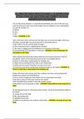
5. Using Figure 17.6, analyze the x objective function coefficient that ranges from a value of 40
to infinity.
Note in Figure 17.6 that an x-coefficient value of infinity causes the objective function to
pivot about point C and to lie along line segment B-C. When the x coefficient is reduced to
40, the objective function lies along the line segment D-C. Further reduction in the value of
the x coefficient would result in a new basic solution with the slack variable 𝑆3 replacing 𝑆1
in the solution. This means the optimal solution will move from extreme point C to D.
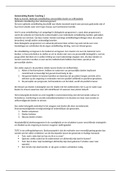
6. Using Figure 17.7, explain what happens to the LP solution as the RHS of binding constraint
2 ranges from $6000 to $9500.
Note in Figure 17.7, that as the RHS of constraint 2 is increased, the extreme point C moves
along line segment C-H until C becomes coincident with H at RHS = 9500. The values of the
basic variables at extreme point H are x = 60, y = 75, 𝑆1 = 0. This is a degenerate solution
because three constraints now define extreme point H. As the RHS value is reduced to 6000,
the extreme point C moves along line segment C-B until C becomes coincident with B at RHS
= 6000. The values of the basic variables at extreme point B are 𝑆1 = 280, 𝑆2 = 2000, and
x = 60.
7. Linear programming is a special case of goal programming. Explain.
Linear programming is a special case of goal programming, because any linear
programming problem can be formulated as a goal programming problem. This is
accomplished by placing the appropriate deviation variables for the constraints at the
+ −
highest priority level (e.g., d deviation variables for constraints and d deviation
variables for constraints). Furthermore, linear programming is less flexible than goal
programming because LP permits only one objective function and all constraints must be
met absolutely.
8. What are some limitations to the use of LP?
An obvious limitation of linear programming is the requirement for integer solutions in
some applications. A more subtle limitation is the art required to formulate complex
problems as linear programs. Linear programming models are rather abstract and
consequently, some managers may resist using them for decision making. No real
computational limitations exist today and linear programming codes are readily available.
EXERCISE SOLUTIONS
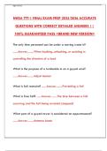
S2.1 (a)
, Let: A = number of gallons of fuel A in the blend
B = number of gallons of fuel B in the blend
Minimize Z = 0.2A + 0.lB
90 A + 75B
= 80 Octane
Subject to: A+ B
(b)
4000
z = 400
3000 2A - B > 0
2000 A < 2000
1000 A + B > 3000
1000 2000 3000 4000
Optimal Solution: A = 1000 gallons
B = 2000 gallons
C = $400
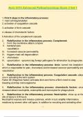
S2.2 Let: Mij = number of minority people from district i who attend school j
Wij = number of white people from district i who attend school j
Dij = distance from district i to school
Minimize Z: ∑7𝑖=1 ∑3𝑗=1 𝐷ij (𝑀ij + 𝑊ij )
Subject to: ∑7𝑖=1(𝑀ij + 𝑊ij ) ≤ 400 for 𝑗 = 1,2,3 school capacity
3
M
j =1
1j = 90
[Create a set of seven equations, one for each
district to ensure that each minority student is
placed in a school.]
3
M
j =1
7j = 10
TEACHING NOTE
In this supplement the analytical technique known as linear programming (LP) is explored.
The emphasis is on developing the student's ability to formulate linear programming
models and to interpret computer output for making decisions. The concept of constrained
optimization models is first developed as a realistic view of many decision problems. An
example problem, Stereo Warehouse, is used throughout the chapter to illustrate the
features of linear programming. Formulating LP models is an art best learned by working
with examples. Therefore, we present a selection of several LP model applications for
services that guide the student through the formulation of the problems. We do not discuss
the simplex algorithm and the mechanics of "pivoting." Instead, we use a graphical and
intuitive approach to explain how optimal solutions are found. Sensitivity analysis is
explained using graphs to illustrate the impact on the solution of ranging objective function
coefficients and right-hand-side (RHS) values. Throughout the discussion, an Excel Solver
Add-in is used to illustrate computer solutions and printouts are displayed and interpreted.
The final section deals with goal programming, which is a popular extension of LP for
dealing with multiple objectives. The example in this section also illustrates how a goal
programming problem with preemptive priorities can be formulated using a typical LP
package.
SUPPLEMENTARY MATERIALS
Case: Red Brand Canners (HBS case 9-110-063)
This very popular case looks at a decision on the mix of tomato products to process and the
assessment of the price to pay for additional tomatoes.
Case: Avis Rent-A-Car System, Inc. (A) (HBS case 9-172-275)
This is a comprehensive case dealing with the Avis fleet planning model.
Excel Solver: Operations Research Add-ins for Microsoft Excel
A selection of Excel Solver programs has been developed by Professor Paul A. Jensen,
Operations Research/Industrial Engineering Program, Department of Mechanical
Engineering, University of Texas at Austin, 1996. The Add-ins are available on the Web at:
http://hawkeye.me.utexas.edu/~jensen/
LECTURE OUTLINE
I. Constrained Optimization Models
II. Formulating Linear Programming Models
, Diet problem
Shift-scheduling problem
Workforce planning problem
Transportation problem
III. Optimal Solutions and Computer Analysis
Graphical solution of LP models
LP model in standard form
Computer analysis and interpretation
IV. Sensitivity Analysis
Objective function coefficient ranges
Right-hand-side (RHS) ranging
V. Goal Programming
TOPICS FOR DISCUSSION
1. Give some everyday examples of constrained optimization problems.
Time is the most common constraint on making everyday decisions. The urgency for
arriving at a solution limits the number of alternatives that can be investigated. Waiting
until the last moment to buy a Christmas present decreases our choices of gifts. Buying a
home is constrained by several factors such as our ability to secure a loan, the number of
homes on the market, and the time we have available to look for housing. Finding a place to
eat lunch is constrained by our budget, the number of restaurants in the area,
transportation available, and the amount of time we can be away from work.
2. How can the validity of LP models be evaluated?
The issue of model validity is divided into internal and external validity. Internal validity is
concerned with the computational correctness of the relationships imbedded in the model.
Internal validity is evaluated by running the model and checking the results by hand-
calculation. External validity concerns the question: Does the model replicate reality?
External validity can be tested by comparing the model outputs to historical data. For
example, does the objective function estimate the relevant operating costs for various
resource allocations used in the past? External validation is also established when the
model generates results that correspond to the decision maker's view of reality.
3. Interpret the meaning of the opportunity cost for a nonbasic decision variable that did not
appear in the LP solution.
The opportunity cost for a nonbasic decision variable, in contrast to a slack or surplus
variable, also has an economic meaning. The opportunity cost represents the undesirable
change in the objective function per unit of the decision variable if this variable is brought
into the solution and thus, is made basic.
,4. Explain graphically what has happened when a degenerate solution occurs in an LP
problem.
A degenerate solution occurs when one or more basic variables has a value of zero. This can
be shown graphically for a two-decision variable problem when an extreme point is defined
by the intersection of more than two constraint equations.
5. Using Figure 17.6, analyze the x objective function coefficient that ranges from a value of 40
to infinity.
Note in Figure 17.6 that an x-coefficient value of infinity causes the objective function to
pivot about point C and to lie along line segment B-C. When the x coefficient is reduced to
40, the objective function lies along the line segment D-C. Further reduction in the value of
the x coefficient would result in a new basic solution with the slack variable 𝑆3 replacing 𝑆1
in the solution. This means the optimal solution will move from extreme point C to D.
6. Using Figure 17.7, explain what happens to the LP solution as the RHS of binding constraint
2 ranges from $6000 to $9500.
Note in Figure 17.7, that as the RHS of constraint 2 is increased, the extreme point C moves
along line segment C-H until C becomes coincident with H at RHS = 9500. The values of the
basic variables at extreme point H are x = 60, y = 75, 𝑆1 = 0. This is a degenerate solution
because three constraints now define extreme point H. As the RHS value is reduced to 6000,
the extreme point C moves along line segment C-B until C becomes coincident with B at RHS
= 6000. The values of the basic variables at extreme point B are 𝑆1 = 280, 𝑆2 = 2000, and
x = 60.
7. Linear programming is a special case of goal programming. Explain.
Linear programming is a special case of goal programming, because any linear
programming problem can be formulated as a goal programming problem. This is
accomplished by placing the appropriate deviation variables for the constraints at the
+ −
highest priority level (e.g., d deviation variables for constraints and d deviation
variables for constraints). Furthermore, linear programming is less flexible than goal
programming because LP permits only one objective function and all constraints must be
met absolutely.
8. What are some limitations to the use of LP?
An obvious limitation of linear programming is the requirement for integer solutions in
some applications. A more subtle limitation is the art required to formulate complex
problems as linear programs. Linear programming models are rather abstract and
consequently, some managers may resist using them for decision making. No real
computational limitations exist today and linear programming codes are readily available.
EXERCISE SOLUTIONS
S2.1 (a)
, Let: A = number of gallons of fuel A in the blend
B = number of gallons of fuel B in the blend
Minimize Z = 0.2A + 0.lB
90 A + 75B
= 80 Octane
Subject to: A+ B
(b)
4000
z = 400
3000 2A - B > 0
2000 A < 2000
1000 A + B > 3000
1000 2000 3000 4000
Optimal Solution: A = 1000 gallons
B = 2000 gallons
C = $400
S2.2 Let: Mij = number of minority people from district i who attend school j
Wij = number of white people from district i who attend school j
Dij = distance from district i to school
Minimize Z: ∑7𝑖=1 ∑3𝑗=1 𝐷ij (𝑀ij + 𝑊ij )
Subject to: ∑7𝑖=1(𝑀ij + 𝑊ij ) ≤ 400 for 𝑗 = 1,2,3 school capacity
3
M
j =1
1j = 90
[Create a set of seven equations, one for each
district to ensure that each minority student is
placed in a school.]
3
M
j =1
7j = 10