Part 1 Opti on Valuati on Methods
Chapter 1 Options/derivative
What are options?
Asset = financial object whose value is known at present but is liable to change in the future
(shares, commodities, currencies).
European call option = gives the holder the right (not obligation) to purchase a prescribed
asset for a prescribed price at a prescribed time in the future from the writer. You expect the
stock price to rise.
Exercise price or strike price (E) = the prescribed purchase price of the asset.
Expiry date = the prescribed time in the future the asset can be bought.
Value of the option = the price you pay for the option.
European put option = gives the holder the right (not obligation) to sell a prescribed asset for
a prescribed price at a prescribed time in the future to the writer. You expect the stock price
to fall.
The key question of the book is: how do we compute a fair option value?
Why do we study options?
Hedge = a strategy to reduce the risk of adverse price movements in an asset.
Portfolio = a collection of options that someone holds.
Two reasons why options are popular: (1) options are attractive to
investors, both for speculation and for hedging; (2) there is a systematic
way to determine how much they are worth.
E = strike price.
S (T) = the price of the asset at the expiry date.
S (t) = the price of the asset over time.
C = the value of a European call option at the expiry date.
C=max (S ( T ) −E , 0)
P = the value of a European put option at the expiry date.
P=max (E−S ( T ) , 0)
Call option: if S(T) > E holder buys asset for E (option) and sells for S(T)
profit = S(T) – E; is E S(T) holder doesn’t buy asset profit = 0.
Put option: if E > S(T) holder buys asset for S(T) and sells for E (option) Figure 1 Payoff diagram for
profit = E – S(T); or S(T) E holder doesn’t buy asset profit = 0. European call and put option
Bottom straddle = hold a call option and put option on the same asset with the same expiry
and strike price. Overall value = ¿ S ( T ) −E∨¿ . Profit when S(T) is far away from E.
Bull spread = hold a call option with E1 and write a call option with E2 for the same asset and
expiry date, where E2 > E1. Overall value = max ( S ( T )−E1 , 0 ) −max ( S ( T )−E2 , 0 ). Profit when
S(T) > E1, but no extra when S(T) > E2.
How are options traded?
Market maker = individuals who are obliged to buy or sell options whenever asked to do so.
Bid = the price at which the market maker will buy the option from you.
Ask = the price at which the market maker will sell the option to you. Ask > Bid.
1
,Bid-ask spread = the difference between the ask and the bid.
Over-the-counter deals = options that are traded between large financial institutions.
Typical option prices
Figure 2 Market values for IBM call and put options for a range of strike prices and times to expiry
Other financial derivatives
Financial derivative = the value is derived from the underlying assets.
Chapter 2 Option valuation preliminaries
Motivation
There are certain simple results about option valuation methods that can be deduced from
first principles. To do this we introduce two key concepts: discounting for interest and no
arbitrage.
Interest rates
Continuously compounded interest rate / annual rate (r) = the amount that a lender charges
for the use of assets expressed as a percentage of the assets. The amount D 0 grows
according to r over a time length t: D ( t ) =e rt D 0. Assumption: there is a fixed interest rate
whenever cash is lent or borrowed.
Discounting for interest / discounting for inflation = determining the present value of a
payment that is received in the future. An amount of €100 at time t will have the value of
€100e rt at time 0. A larger discount creates a greater return, which is a function of risk.
Short selling
Short selling = selling an item that is now owned with the intention of buying it back at a
later date. You must first borrow the item from someone who owns it and give it back later.
The overall profit/loss at time t = t2 is: e r (t −t ) S (t 1)−S (t 2) (t1 is the time of the sell, t2 is the
2 1
time of the buy and give back).
Arbitrage
Option valuation theory rests on no arbitrage = there is never an opportunity to make a risk-
free profit that gives a greater return than that provided by the interest from a bank deposit.
This is because investors would borrow money from a bank and spend it on a risk-free
portfolio. The supply and demand would cause the profit from the portfolio to drop or the
interest rate to increase.
2
,Put-call parity
Put-call parity = the relationship between a European call option and a European put option:
−rT
C+ E e =P+ S
Upper and lower bounds on option values
According to the no arbitrage principle: a portfolio with a higher maximum payoff can never
have a lower time-zero value than a portfolio with a lower maximum payoff.
The upper and lower bounds for the value of a European call option at expiry are:
C ≥ max ( S−E e ,0 ) and C ≤ S
−rT
The upper and lower bounds for the value of a European put option at expiry are:
P ≥ max ( E e−rT −S , 0 ) and P ≤ E e−rT
Example
Two European call options with expiry dates T 1 and T 2, with T 2>T 1 and the same strike price
E . Suppose the holder of the option with T 2 takes the following actions at t=T 1:
1. If S(T 1) ≤ E , do nothing because the T 1 option will have zero payoff, so the T 2 will
do no better.
2. If S ( T 1) > E, the short sell one unit of the asset, invest the money and buy the asset
back at t=T 2 because the holder of the T 2 option hedges against the possibility of
the fall of the stock price by investing the profit of the short sell risk-free.
In case 1, the holder of the T 2 option will have an overall profit of
r ( T −T )
e 2 1
max( S ( T 1 )−E , 0 ¿=0. In case 2, the holder of the T 2 option will have a profit of max ¿
S( T 2 )−E , 0 ¿ (original T 2 option) + e (
r T −T )
S(T 1 ) (reinvesting the profits of the short sell)
2 1
−S(T 2) (buying the asset back for the short sell. The overall payoff for case 2 is:
r (T −T )
max ( S ( T 2 )−E ,0 ) +e S ( T 1 )−S ( T 2)
2 1
r (T 2−T 1) r (T 2 −T 1)
¿ max (e S ( T 1 ) −E , e S ( T 1 ) −S ( T 2 ) )
r (T 2−T 1) r ( T 2−T 1)
≥e (S ( T 1 )−E)=e max( S ( T 1 )−E ,0)
Chapter 3 Random variables
Random variables, probability and mean
Types of random variables: discrete and continuous. Discrete random variables have a finite
list of outcomes, which all have a positive probability which add up to 1. Continuous random
variables are measurements (infinite), which all have a positive probability that add up to 1:
∞
∫ f ( a ) da ( f ( a ) is the probability density function).
−∞
P( X=x i) means the probability that X =x i. This is only possible when there are no negative
m
probabilities and when all the probabilities add up to 1: pi ≥0 for all i; ∑ pi=1 .
i=1
The mean or expected value ( E , μ) is denoted by:
m
E ( X ) ≔ ∑ x i pi
i=1
3
, For a Bernoulli random variable with parameter p, the random variable X is 1 with a
probability of 0 ≤ p ≤ 1 and it is 0 with a probability of 1− p . This gives:
E ( X ) =1 p+0 ( 1−p )= p
The probability for a continuous random variable R is found via the density function:
b ∞
P ( a ≤ X ≤ b )=∫ f ( x ) dx where f ( x ) ≥ 0 for all x and ∫ f ( x ) dx=1
a −∞
The mean or the expected value of a continuous random variable X is:
∞
E ( X ) ≔ ∫ xf ( x ) dx
−∞
The mean of the sums is the same as the sum of the means, and the mean scales linearly:
E ( X +Y ) =E ( X ) + E(Y )
E ( αX )=α E (X ) for α ∈ R
0
f ( x )=
{
( β−α )−1 , for α< x < β ,
otherwise
The function above has a uniform distribution over ( α , β ) → X ⋃(α , β), which means that X
only takes values between α and β . The mean of this function is given by
So, if we apply a function h to a continuous random variable X, then the mean of the random
variable h(X) is given by:
∞
E ( h ( X )) =∫ h ( x ) f ( x ) dx
−∞
Independence
When two variables X and Y are independent, this means that they do not depend on each
other: E ( g ( X ) h ( Y ) )=E (g ( X ) ) E(h (Y )) for all g , h :R → R. X and Y are independent
⟹ E ( XY )=E ( X )E(Y ) .
Sequences of random variables that are independent and identically distributed (i.i.d) = in the
discrete case the Xi have the same possible values (x1, …, xm) and probabilities (p1, …, pm); and
in the continuous case the Xi have the same density function. Being told any values of the Xi’s
doesn’t tell us anything about the other Xi’s.
Variance
Variance (V , σ 2) = the variation that the values of Xi has around the mean value.
V ( X ) ≔ E (( X−E ( X ) ) ) ≔ E ( X )−( E ( X ) ) . Var ( αX )=α 2 Var ( X ).
2 2 2
The standard deviation (std, σ ) is defined as: std ( X ) ≔ √ Var ( X) .
Normal distribution
When X has a standard normal distribution X N ( μ , σ 2 ) it is characterised with the density
function with μ is the mean and σ 2 is the variance:
2
− ( x− μ)
1 2σ
2
f ( x )= e
√2 π σ 2
4
Chapter 1 Options/derivative
What are options?
Asset = financial object whose value is known at present but is liable to change in the future
(shares, commodities, currencies).
European call option = gives the holder the right (not obligation) to purchase a prescribed
asset for a prescribed price at a prescribed time in the future from the writer. You expect the
stock price to rise.
Exercise price or strike price (E) = the prescribed purchase price of the asset.
Expiry date = the prescribed time in the future the asset can be bought.
Value of the option = the price you pay for the option.
European put option = gives the holder the right (not obligation) to sell a prescribed asset for
a prescribed price at a prescribed time in the future to the writer. You expect the stock price
to fall.
The key question of the book is: how do we compute a fair option value?
Why do we study options?
Hedge = a strategy to reduce the risk of adverse price movements in an asset.
Portfolio = a collection of options that someone holds.
Two reasons why options are popular: (1) options are attractive to
investors, both for speculation and for hedging; (2) there is a systematic
way to determine how much they are worth.
E = strike price.
S (T) = the price of the asset at the expiry date.
S (t) = the price of the asset over time.
C = the value of a European call option at the expiry date.
C=max (S ( T ) −E , 0)
P = the value of a European put option at the expiry date.
P=max (E−S ( T ) , 0)
Call option: if S(T) > E holder buys asset for E (option) and sells for S(T)
profit = S(T) – E; is E S(T) holder doesn’t buy asset profit = 0.
Put option: if E > S(T) holder buys asset for S(T) and sells for E (option) Figure 1 Payoff diagram for
profit = E – S(T); or S(T) E holder doesn’t buy asset profit = 0. European call and put option
Bottom straddle = hold a call option and put option on the same asset with the same expiry
and strike price. Overall value = ¿ S ( T ) −E∨¿ . Profit when S(T) is far away from E.
Bull spread = hold a call option with E1 and write a call option with E2 for the same asset and
expiry date, where E2 > E1. Overall value = max ( S ( T )−E1 , 0 ) −max ( S ( T )−E2 , 0 ). Profit when
S(T) > E1, but no extra when S(T) > E2.
How are options traded?
Market maker = individuals who are obliged to buy or sell options whenever asked to do so.
Bid = the price at which the market maker will buy the option from you.
Ask = the price at which the market maker will sell the option to you. Ask > Bid.
1
,Bid-ask spread = the difference between the ask and the bid.
Over-the-counter deals = options that are traded between large financial institutions.
Typical option prices
Figure 2 Market values for IBM call and put options for a range of strike prices and times to expiry
Other financial derivatives
Financial derivative = the value is derived from the underlying assets.
Chapter 2 Option valuation preliminaries
Motivation
There are certain simple results about option valuation methods that can be deduced from
first principles. To do this we introduce two key concepts: discounting for interest and no
arbitrage.
Interest rates
Continuously compounded interest rate / annual rate (r) = the amount that a lender charges
for the use of assets expressed as a percentage of the assets. The amount D 0 grows
according to r over a time length t: D ( t ) =e rt D 0. Assumption: there is a fixed interest rate
whenever cash is lent or borrowed.
Discounting for interest / discounting for inflation = determining the present value of a
payment that is received in the future. An amount of €100 at time t will have the value of
€100e rt at time 0. A larger discount creates a greater return, which is a function of risk.
Short selling
Short selling = selling an item that is now owned with the intention of buying it back at a
later date. You must first borrow the item from someone who owns it and give it back later.
The overall profit/loss at time t = t2 is: e r (t −t ) S (t 1)−S (t 2) (t1 is the time of the sell, t2 is the
2 1
time of the buy and give back).
Arbitrage
Option valuation theory rests on no arbitrage = there is never an opportunity to make a risk-
free profit that gives a greater return than that provided by the interest from a bank deposit.
This is because investors would borrow money from a bank and spend it on a risk-free
portfolio. The supply and demand would cause the profit from the portfolio to drop or the
interest rate to increase.
2
,Put-call parity
Put-call parity = the relationship between a European call option and a European put option:
−rT
C+ E e =P+ S
Upper and lower bounds on option values
According to the no arbitrage principle: a portfolio with a higher maximum payoff can never
have a lower time-zero value than a portfolio with a lower maximum payoff.
The upper and lower bounds for the value of a European call option at expiry are:
C ≥ max ( S−E e ,0 ) and C ≤ S
−rT
The upper and lower bounds for the value of a European put option at expiry are:
P ≥ max ( E e−rT −S , 0 ) and P ≤ E e−rT
Example
Two European call options with expiry dates T 1 and T 2, with T 2>T 1 and the same strike price
E . Suppose the holder of the option with T 2 takes the following actions at t=T 1:
1. If S(T 1) ≤ E , do nothing because the T 1 option will have zero payoff, so the T 2 will
do no better.
2. If S ( T 1) > E, the short sell one unit of the asset, invest the money and buy the asset
back at t=T 2 because the holder of the T 2 option hedges against the possibility of
the fall of the stock price by investing the profit of the short sell risk-free.
In case 1, the holder of the T 2 option will have an overall profit of
r ( T −T )
e 2 1
max( S ( T 1 )−E , 0 ¿=0. In case 2, the holder of the T 2 option will have a profit of max ¿
S( T 2 )−E , 0 ¿ (original T 2 option) + e (
r T −T )
S(T 1 ) (reinvesting the profits of the short sell)
2 1
−S(T 2) (buying the asset back for the short sell. The overall payoff for case 2 is:
r (T −T )
max ( S ( T 2 )−E ,0 ) +e S ( T 1 )−S ( T 2)
2 1
r (T 2−T 1) r (T 2 −T 1)
¿ max (e S ( T 1 ) −E , e S ( T 1 ) −S ( T 2 ) )
r (T 2−T 1) r ( T 2−T 1)
≥e (S ( T 1 )−E)=e max( S ( T 1 )−E ,0)
Chapter 3 Random variables
Random variables, probability and mean
Types of random variables: discrete and continuous. Discrete random variables have a finite
list of outcomes, which all have a positive probability which add up to 1. Continuous random
variables are measurements (infinite), which all have a positive probability that add up to 1:
∞
∫ f ( a ) da ( f ( a ) is the probability density function).
−∞
P( X=x i) means the probability that X =x i. This is only possible when there are no negative
m
probabilities and when all the probabilities add up to 1: pi ≥0 for all i; ∑ pi=1 .
i=1
The mean or expected value ( E , μ) is denoted by:
m
E ( X ) ≔ ∑ x i pi
i=1
3
, For a Bernoulli random variable with parameter p, the random variable X is 1 with a
probability of 0 ≤ p ≤ 1 and it is 0 with a probability of 1− p . This gives:
E ( X ) =1 p+0 ( 1−p )= p
The probability for a continuous random variable R is found via the density function:
b ∞
P ( a ≤ X ≤ b )=∫ f ( x ) dx where f ( x ) ≥ 0 for all x and ∫ f ( x ) dx=1
a −∞
The mean or the expected value of a continuous random variable X is:
∞
E ( X ) ≔ ∫ xf ( x ) dx
−∞
The mean of the sums is the same as the sum of the means, and the mean scales linearly:
E ( X +Y ) =E ( X ) + E(Y )
E ( αX )=α E (X ) for α ∈ R
0
f ( x )=
{
( β−α )−1 , for α< x < β ,
otherwise
The function above has a uniform distribution over ( α , β ) → X ⋃(α , β), which means that X
only takes values between α and β . The mean of this function is given by
So, if we apply a function h to a continuous random variable X, then the mean of the random
variable h(X) is given by:
∞
E ( h ( X )) =∫ h ( x ) f ( x ) dx
−∞
Independence
When two variables X and Y are independent, this means that they do not depend on each
other: E ( g ( X ) h ( Y ) )=E (g ( X ) ) E(h (Y )) for all g , h :R → R. X and Y are independent
⟹ E ( XY )=E ( X )E(Y ) .
Sequences of random variables that are independent and identically distributed (i.i.d) = in the
discrete case the Xi have the same possible values (x1, …, xm) and probabilities (p1, …, pm); and
in the continuous case the Xi have the same density function. Being told any values of the Xi’s
doesn’t tell us anything about the other Xi’s.
Variance
Variance (V , σ 2) = the variation that the values of Xi has around the mean value.
V ( X ) ≔ E (( X−E ( X ) ) ) ≔ E ( X )−( E ( X ) ) . Var ( αX )=α 2 Var ( X ).
2 2 2
The standard deviation (std, σ ) is defined as: std ( X ) ≔ √ Var ( X) .
Normal distribution
When X has a standard normal distribution X N ( μ , σ 2 ) it is characterised with the density
function with μ is the mean and σ 2 is the variance:
2
− ( x− μ)
1 2σ
2
f ( x )= e
√2 π σ 2
4