VITTORIO CESCHI’S LECTURES SUMMARY
CM1005-Introduction to Statistical Analysis
Lecture summary
Week 1
Three main categories for classifying statistics (refers to how many variable you deal with in
your analysis):
• Univariate: What was the average grade of the ISA exam last year? We’re gonna
measure just one variable:
grade
• Bivariate: Did males and females differ in their grades? Two variables are
interrelated:
gender → grade
• Multivariate: What was the grade dependent on initial motivation, the time spent on
reading and gender? Different variables relating to another variable:
Motivation - time spent - gender → grade
Statistics: “The study of how we describe and make inferences from data.” (Sirkin)
➢ Distinction between descriptive & inferential statistics
➢ An inference is “a conclusion reached on the basis of evidence and reasoning” – i.e.
making a statement and gaining statistics about a population using your sample –
deals with a population
➢ Descriptive statistics is more taking direct measurement of your data – i.e. just
measuring your sample and making statistics on your sample
Unit of analysis: “the what or who that is being studied”
➢ The unit that you will be able to draw conclusions about
➢ What are the units contained in our dataset?
➢ Typically, all units are the same type of thing in a single data set
Variable: a measured property of each of the units of analysis
Levels of measurement:
➢ Nominal: group categorization; no meaningful ranking possible (one is just different
than the other); numerical coding arbitrary (can appear in different order)
➢ Ordinal: meaningful ranking along a given dimension (i.e. strongly agree, agree,
neutral, not agree, strongly not agree) but, distance between categories is not equal
(difference between 1 and 2 is not equal to difference between 2 and 3)
Nominal and Ordinal are more qualitative
➢ Interval: meaningful ranking; distances are equal, doesn’t have a meaningful zero
point (difference between 15 and 17 is equal to difference between 20 and 22)
➢ Ratio: all properties of interval (ranking and equal distances); absolute and
meaningful zero point
Interval and Ratio are more quantitative
1
,We always need to know the level of measurement in order to know which statistical
techniques we may use for the given variable.
Continuous vs Discrete variables: “A continuous variable is measured along a continuum
(a number that can have a decimal point i.e. 3,8), whereas a discrete variable is measured in
whole units or categories (wouldn’t have a fractional part)”
Measures of central tendency: to (univariately) describe the distribution of variables
on different levels of measurement
• A first measure of central tendency: the mean/average)
➢ i.e. Measuring trust in the news media
(on a 11 points scale, 0=no trust; 10=complete trust)
10 respondents in our sample (n = 10)
What is the average (mean) trust in the news media in this sample?
- We write the sample mean as M
- All values are added up and divided by n; i.e. the number of observations in the
sample
- ∑ = Capital greek sigma, meaning the sum of something
- Almost same formula for the population mean
Some characteristics of the mean:
• Changing any score will change the mean
• Adding or removing a score will change mean (unless that score is already equal to
mean)
• Adding, subtracting, multiplying, dividing each score by a given value causes the
mean to change accordingly
• Sum of differences from the mean is zero (has to be true)
• Sum of squared differences from the mean is minimal (we square – alla seconda – the
result of the parenthesis (x-M))
➢ The result (42 in this case) is also called Sum of Squares (SS)
➢ For now, a larger SS means that scores deviate more from the mean
➢ Why “minimal”? – If we had used any other value than the mean (5) to
calculate the SS, it would have been larger than 42
• A second measure of central tendency: the median/middle point (ordinal &
interval/ratio)
➢ i.e. Measuring income (n=9)
1= less than 500
2=501-1000
2
, 3=1001-1500
4=1501-2000
5=2001-3000
6=more than 3000
To find the median:
1) Sort all cases based on their value on x
2) The value of the “middle case” equals the median (equal amount of cases/observations
below and above)
➢ If n is an even (pari) number, the median is the mean value of the two
middle cases
Frequency tables in SPSS:
➢ Frequency: refers to how many of each thing
➢ To determine the median from a frequency table, we need to identify
the first category that exceeds 50% in the “cumulative percent”
column
• A third measure of central tendency: the mode (nominal, ordinal, interval/ratio)
➢ The mode is the category with the largest amount of cases/frequency
➢ i.e. Religion (n=9)
1=Atheist
2=Protestant
3=Catholic
4=Muslim
5=Other
Our sample: (1;3;2;2;2;5;1;2;4)
In this case the mode is 2 (Protestant)
3
, This above is a skewed distribution
4
CM1005-Introduction to Statistical Analysis
Lecture summary
Week 1
Three main categories for classifying statistics (refers to how many variable you deal with in
your analysis):
• Univariate: What was the average grade of the ISA exam last year? We’re gonna
measure just one variable:
grade
• Bivariate: Did males and females differ in their grades? Two variables are
interrelated:
gender → grade
• Multivariate: What was the grade dependent on initial motivation, the time spent on
reading and gender? Different variables relating to another variable:
Motivation - time spent - gender → grade
Statistics: “The study of how we describe and make inferences from data.” (Sirkin)
➢ Distinction between descriptive & inferential statistics
➢ An inference is “a conclusion reached on the basis of evidence and reasoning” – i.e.
making a statement and gaining statistics about a population using your sample –
deals with a population
➢ Descriptive statistics is more taking direct measurement of your data – i.e. just
measuring your sample and making statistics on your sample
Unit of analysis: “the what or who that is being studied”
➢ The unit that you will be able to draw conclusions about
➢ What are the units contained in our dataset?
➢ Typically, all units are the same type of thing in a single data set
Variable: a measured property of each of the units of analysis
Levels of measurement:
➢ Nominal: group categorization; no meaningful ranking possible (one is just different
than the other); numerical coding arbitrary (can appear in different order)
➢ Ordinal: meaningful ranking along a given dimension (i.e. strongly agree, agree,
neutral, not agree, strongly not agree) but, distance between categories is not equal
(difference between 1 and 2 is not equal to difference between 2 and 3)
Nominal and Ordinal are more qualitative
➢ Interval: meaningful ranking; distances are equal, doesn’t have a meaningful zero
point (difference between 15 and 17 is equal to difference between 20 and 22)
➢ Ratio: all properties of interval (ranking and equal distances); absolute and
meaningful zero point
Interval and Ratio are more quantitative
1
,We always need to know the level of measurement in order to know which statistical
techniques we may use for the given variable.
Continuous vs Discrete variables: “A continuous variable is measured along a continuum
(a number that can have a decimal point i.e. 3,8), whereas a discrete variable is measured in
whole units or categories (wouldn’t have a fractional part)”
Measures of central tendency: to (univariately) describe the distribution of variables
on different levels of measurement
• A first measure of central tendency: the mean/average)
➢ i.e. Measuring trust in the news media
(on a 11 points scale, 0=no trust; 10=complete trust)
10 respondents in our sample (n = 10)
What is the average (mean) trust in the news media in this sample?
- We write the sample mean as M
- All values are added up and divided by n; i.e. the number of observations in the
sample
- ∑ = Capital greek sigma, meaning the sum of something
- Almost same formula for the population mean
Some characteristics of the mean:
• Changing any score will change the mean
• Adding or removing a score will change mean (unless that score is already equal to
mean)
• Adding, subtracting, multiplying, dividing each score by a given value causes the
mean to change accordingly
• Sum of differences from the mean is zero (has to be true)
• Sum of squared differences from the mean is minimal (we square – alla seconda – the
result of the parenthesis (x-M))
➢ The result (42 in this case) is also called Sum of Squares (SS)
➢ For now, a larger SS means that scores deviate more from the mean
➢ Why “minimal”? – If we had used any other value than the mean (5) to
calculate the SS, it would have been larger than 42
• A second measure of central tendency: the median/middle point (ordinal &
interval/ratio)
➢ i.e. Measuring income (n=9)
1= less than 500
2=501-1000
2
, 3=1001-1500
4=1501-2000
5=2001-3000
6=more than 3000
To find the median:
1) Sort all cases based on their value on x
2) The value of the “middle case” equals the median (equal amount of cases/observations
below and above)
➢ If n is an even (pari) number, the median is the mean value of the two
middle cases
Frequency tables in SPSS:
➢ Frequency: refers to how many of each thing
➢ To determine the median from a frequency table, we need to identify
the first category that exceeds 50% in the “cumulative percent”
column
• A third measure of central tendency: the mode (nominal, ordinal, interval/ratio)
➢ The mode is the category with the largest amount of cases/frequency
➢ i.e. Religion (n=9)
1=Atheist
2=Protestant
3=Catholic
4=Muslim
5=Other
Our sample: (1;3;2;2;2;5;1;2;4)
In this case the mode is 2 (Protestant)
3
, This above is a skewed distribution
4