Week 4: Mixed Designs and MANOVA
Ch. 16: Mixed Designs
Mixed Designs
Mixed designs => combine repeated-measures and independent designs
A design that includes some independent variables (1) measured using different
entities and (2) others measured using repeated measures
A mixed design => requires at least two IVs
Assumptions in Mixed Designs
Since we’re using the liner model => all sources of potential bias discussed previously still
apply
Including both (1) homogeneity of variance and (2) sphericity
Sphericity => simply apply the Greenhouse-Geisser correction
Speed-Dating Study Example
Each participant attending a speed-dating night would be exposed to all combinations of
attractiveness and charisma – these are repeated measures
The two repeated-measured variables => Looks (with three levels: attractive,
average, unattractive) and Charisma (with three levels: high charisma, some
charisma, none)
In addition => the ‘date’ employed a hard to get strategy for half of the participants – and
acted normal for the rest
Therefore, Strategy is the
between-group variable
Mixed Designs Using SPSS
,The process for analyzing mixed designs is as follows:
Fitting the Model
The 1st variable Looks has three conditions => (1) attractive, (2) average, (3) unattractive
It makes sense to compare the attractive and unattractive conditions to the average =>
as the average person represents the norm
This comparison could be done using a simple contrast => assigning average to the
1st or last level
The 2nd variable Charisma has a category that represents the norm => some charisma
This category can be used as control against which to compare the two extremes
(high charisma and none)
We can use a simple contrast to compare everything against some charism =>
assigning this category to the 1st or last level
Based on the proposed contrasts => makes sense to have average
as Level 3 of Looks – and some charisma as Level 3 of Charisma
The remaining levels can be assigned arbitrarily:
- Level 1 = attractive; Level 2 = unattractive
, - Level 1 = high charisma; Level 2 = none
Once the levels have been correctly entered => need to place Strategy variable in the
Between-Subjects Factors box
Since we need to specify the between-group variables in a mixed design
Output for Mixed Factorial Designs
The table lists the repeated-measures
variables and the level of each IV that
they represent => useful when need to
remind oneself of what the contrast
levels represent
The second table => contains the
descriptive statistics (M, SD) for each of the nine repeated measures conditions – split
according to whether participants sat with dates who played hard to get or not (= Strategy)
,The information about sphericity for each of the three repeated-measures effects in the model
is shown by the test of sphericity
The Huynh-Feldt estimates are all = 1 which equates to spherical data
No deviation from sphericity is shown by H-F => reasonable not to correct for it
Correcting (using G-G) would have little impact since all the G-G estimates are close
to 1 => may as well correct anyways
The table on the left shows the F-
statistics => this table has been
formatted such that it hides the values
we are not interested in
The table is split into sections for
each of the effects in the model and
their associated error terms
The table also includes the interactions b/n the between-groups variable Strategy and the
repeated-measures effects
It appears that all of the effects are stat significant (=> normally would not be interested in
main effects if there are significant interactions – but all effects will be interpreted anyhow)
Main Effect of Strategy
Levene’s test of equality of error variances => shows
that the variances are homogeneous for all levels of the
repeated-measures variables (p > .05)
,Testing whether the variances were equivalent in the hard to get and normal conditions
across all nine combined levels of the repeated-measures variables
The main
effect of Strategy is listed separately from the repeated-measures effects in the output above
It had a non-sig effect on ratings of dates (p = .946)
This effect indicates that if all other variables are ignored => ratings were equivalent
regardless of whether the data adopted a hard to get or normal persona
The Estimated Marginal Means table – and the plot of these means => indicate that overall,
the ratings of dates playing hard to get were equivalent to dates who acted normal
Main Effect of Looks
The Tests of Within-Subjects Variables => showed a significant main effect of Looks, F(1.92,
34.62) = 423.74, p < .001
Indicates that if all other variables are ignored => ratings of attractive, average and
unattractive dates differed
,The
Estimated Marginal Means and the plot of these means is shown above => showing that as
attractiveness falls, the mean rating falls as well
The levels of Looks are labelled as 1 (attractive), 2 (unattractive), and 3 (average)
The main effect => reflects that the raters were more likely to express a greater interest in
going out with attractive people – than with average or unattractive people
- Contrasts will help understand exactly what is going on
The requested contrasts shown above => interested in the row labelled Looks
The contrast carried out was a simple contrast:
Comparing Level 1 to Level 3 (attractive vs average)
, Then, comparing Level 2 to Level 3 (unattractive vs average)
The values of F for each contrast and their related sig values => indicate that the main effect
of Looks represented the fact that:
1) Attractive dates were rated significantly higher than average dates, F(1, 18) = 226.99,
p < .001
2) Average dates were rated sig higher than unattractive ones, F(1, 18) = 160.07, p
< .001
Main Effect of Charisma
The initial output revealed there was a sig main effect of charisma, F(1.87, 33.62) = 328.25, p
< .002
If all other variables are ignored => ratings for dates with high charisma, some
charisma, and none of it differed
The estimated marginal means and the plot of these means is shown above
The levels of Charisma are labelled as 1 (high), 2 (none), and 3 (some)
The main effect => reflects that as Charisma declines, the mean rating of the date also
declines
, - Raters expressed a greater interest in going out with charismatic people than
average people or those with no charisma
The simple contrast for Charisma => the contrasts represent:
Level 1 vs Level 3 (high vs some)
Level 2 vs Level 3 (none vs some)
These contrasts reveal that the main effect for Charisma is that => highly charismatic dates
were rated sig higher than dates with some charisma, F(1, 18) = 109.94, p < 0.001
- And dates with some charisma were rated sig higher than those with none, F(1,
18) = 227.94, p < 0.001
The Interaction Between Strategy and Looks
Strategy significantly interaction with Looks of the date, F(1.92, 34.62) = 80.43, p < 0.001
The profile or ratings across dates of different attractiveness was different =>
depending on whether or not they played hard to get
The estimated marginal means and interaction graph are shown below:
The graph shows that for
average looks => Strategy does
not make a difference (blue
and orange dots are in similar
location)
For attractive dates => ratings
were higher when the date plays hard to get (= blue dot) compared to when they did not (=
orange dot)
, For the unattractive dates => the opposite pattern is demonstrated
Playing hard to get has an effect only at the extremes of Looks
Another way to look at this is the slope of the lines => when dates played hard to get, the
slope (blue line) is steeper – than when they did not (orange line)
Implying that Looks have a greater impact on ratings when dates play hard to get
This interaction can be clarified using the contrasts:
The 1st contrast for the interaction term => looks at Level 1 of Looks (= attractive) compared
to Level 3 (= average)
- Comparing playing hard to get to normal
The contrast is highly significant, F(1, 18) = 43.26, p < 0.001,
Suggesting that the increased interest in Attractive dates
compared to average-looking dates found when dates play
hard to get => is significantly more than when dates acted
normal
The slope of the blue line (hard to get) b/n attractive dates and
average dates is steeper => in comparison to the orange line (normal)
The preferences for attractive vs average dates => greater when they play hard to get
than when they act normal
Contrast 2 => compares playing hard to get to normal at Level 2 of Looks (= unattractive)
relative to Level 3 (= average) – and is also significant, F(1, 18) = 30.23, p < 0.001
The decreased interest in unattractive vs average-looking dates
when playing hard to get => is significantly more than when
they acted normal
The slope of the blue line b/n the unattractive and average
dates is steeper – than the corresponding orange line
The preferences for average-looking dates compared to
unattractive dates => greater when they play hard to get than when they act normal
Ch. 16: Mixed Designs
Mixed Designs
Mixed designs => combine repeated-measures and independent designs
A design that includes some independent variables (1) measured using different
entities and (2) others measured using repeated measures
A mixed design => requires at least two IVs
Assumptions in Mixed Designs
Since we’re using the liner model => all sources of potential bias discussed previously still
apply
Including both (1) homogeneity of variance and (2) sphericity
Sphericity => simply apply the Greenhouse-Geisser correction
Speed-Dating Study Example
Each participant attending a speed-dating night would be exposed to all combinations of
attractiveness and charisma – these are repeated measures
The two repeated-measured variables => Looks (with three levels: attractive,
average, unattractive) and Charisma (with three levels: high charisma, some
charisma, none)
In addition => the ‘date’ employed a hard to get strategy for half of the participants – and
acted normal for the rest
Therefore, Strategy is the
between-group variable
Mixed Designs Using SPSS
,The process for analyzing mixed designs is as follows:
Fitting the Model
The 1st variable Looks has three conditions => (1) attractive, (2) average, (3) unattractive
It makes sense to compare the attractive and unattractive conditions to the average =>
as the average person represents the norm
This comparison could be done using a simple contrast => assigning average to the
1st or last level
The 2nd variable Charisma has a category that represents the norm => some charisma
This category can be used as control against which to compare the two extremes
(high charisma and none)
We can use a simple contrast to compare everything against some charism =>
assigning this category to the 1st or last level
Based on the proposed contrasts => makes sense to have average
as Level 3 of Looks – and some charisma as Level 3 of Charisma
The remaining levels can be assigned arbitrarily:
- Level 1 = attractive; Level 2 = unattractive
, - Level 1 = high charisma; Level 2 = none
Once the levels have been correctly entered => need to place Strategy variable in the
Between-Subjects Factors box
Since we need to specify the between-group variables in a mixed design
Output for Mixed Factorial Designs
The table lists the repeated-measures
variables and the level of each IV that
they represent => useful when need to
remind oneself of what the contrast
levels represent
The second table => contains the
descriptive statistics (M, SD) for each of the nine repeated measures conditions – split
according to whether participants sat with dates who played hard to get or not (= Strategy)
,The information about sphericity for each of the three repeated-measures effects in the model
is shown by the test of sphericity
The Huynh-Feldt estimates are all = 1 which equates to spherical data
No deviation from sphericity is shown by H-F => reasonable not to correct for it
Correcting (using G-G) would have little impact since all the G-G estimates are close
to 1 => may as well correct anyways
The table on the left shows the F-
statistics => this table has been
formatted such that it hides the values
we are not interested in
The table is split into sections for
each of the effects in the model and
their associated error terms
The table also includes the interactions b/n the between-groups variable Strategy and the
repeated-measures effects
It appears that all of the effects are stat significant (=> normally would not be interested in
main effects if there are significant interactions – but all effects will be interpreted anyhow)
Main Effect of Strategy
Levene’s test of equality of error variances => shows
that the variances are homogeneous for all levels of the
repeated-measures variables (p > .05)
,Testing whether the variances were equivalent in the hard to get and normal conditions
across all nine combined levels of the repeated-measures variables
The main
effect of Strategy is listed separately from the repeated-measures effects in the output above
It had a non-sig effect on ratings of dates (p = .946)
This effect indicates that if all other variables are ignored => ratings were equivalent
regardless of whether the data adopted a hard to get or normal persona
The Estimated Marginal Means table – and the plot of these means => indicate that overall,
the ratings of dates playing hard to get were equivalent to dates who acted normal
Main Effect of Looks
The Tests of Within-Subjects Variables => showed a significant main effect of Looks, F(1.92,
34.62) = 423.74, p < .001
Indicates that if all other variables are ignored => ratings of attractive, average and
unattractive dates differed
,The
Estimated Marginal Means and the plot of these means is shown above => showing that as
attractiveness falls, the mean rating falls as well
The levels of Looks are labelled as 1 (attractive), 2 (unattractive), and 3 (average)
The main effect => reflects that the raters were more likely to express a greater interest in
going out with attractive people – than with average or unattractive people
- Contrasts will help understand exactly what is going on
The requested contrasts shown above => interested in the row labelled Looks
The contrast carried out was a simple contrast:
Comparing Level 1 to Level 3 (attractive vs average)
, Then, comparing Level 2 to Level 3 (unattractive vs average)
The values of F for each contrast and their related sig values => indicate that the main effect
of Looks represented the fact that:
1) Attractive dates were rated significantly higher than average dates, F(1, 18) = 226.99,
p < .001
2) Average dates were rated sig higher than unattractive ones, F(1, 18) = 160.07, p
< .001
Main Effect of Charisma
The initial output revealed there was a sig main effect of charisma, F(1.87, 33.62) = 328.25, p
< .002
If all other variables are ignored => ratings for dates with high charisma, some
charisma, and none of it differed
The estimated marginal means and the plot of these means is shown above
The levels of Charisma are labelled as 1 (high), 2 (none), and 3 (some)
The main effect => reflects that as Charisma declines, the mean rating of the date also
declines
, - Raters expressed a greater interest in going out with charismatic people than
average people or those with no charisma
The simple contrast for Charisma => the contrasts represent:
Level 1 vs Level 3 (high vs some)
Level 2 vs Level 3 (none vs some)
These contrasts reveal that the main effect for Charisma is that => highly charismatic dates
were rated sig higher than dates with some charisma, F(1, 18) = 109.94, p < 0.001
- And dates with some charisma were rated sig higher than those with none, F(1,
18) = 227.94, p < 0.001
The Interaction Between Strategy and Looks
Strategy significantly interaction with Looks of the date, F(1.92, 34.62) = 80.43, p < 0.001
The profile or ratings across dates of different attractiveness was different =>
depending on whether or not they played hard to get
The estimated marginal means and interaction graph are shown below:
The graph shows that for
average looks => Strategy does
not make a difference (blue
and orange dots are in similar
location)
For attractive dates => ratings
were higher when the date plays hard to get (= blue dot) compared to when they did not (=
orange dot)
, For the unattractive dates => the opposite pattern is demonstrated
Playing hard to get has an effect only at the extremes of Looks
Another way to look at this is the slope of the lines => when dates played hard to get, the
slope (blue line) is steeper – than when they did not (orange line)
Implying that Looks have a greater impact on ratings when dates play hard to get
This interaction can be clarified using the contrasts:
The 1st contrast for the interaction term => looks at Level 1 of Looks (= attractive) compared
to Level 3 (= average)
- Comparing playing hard to get to normal
The contrast is highly significant, F(1, 18) = 43.26, p < 0.001,
Suggesting that the increased interest in Attractive dates
compared to average-looking dates found when dates play
hard to get => is significantly more than when dates acted
normal
The slope of the blue line (hard to get) b/n attractive dates and
average dates is steeper => in comparison to the orange line (normal)
The preferences for attractive vs average dates => greater when they play hard to get
than when they act normal
Contrast 2 => compares playing hard to get to normal at Level 2 of Looks (= unattractive)
relative to Level 3 (= average) – and is also significant, F(1, 18) = 30.23, p < 0.001
The decreased interest in unattractive vs average-looking dates
when playing hard to get => is significantly more than when
they acted normal
The slope of the blue line b/n the unattractive and average
dates is steeper – than the corresponding orange line
The preferences for average-looking dates compared to
unattractive dates => greater when they play hard to get than when they act normal