LECTURE 3: LINEAIR REGRESSION
MULTIPLE REGRESSION ANALYSE: DE BASIS
• Meerdere predictoren X1, X2…. Xk
• Yi =b0 +b1Xi1 +b2Xi2 +...+ei
Several regression coefficients bj
bj = expected increase in Y with a 1-point increase in Xj (predictor) ,while keeping the other
predictors constant
ELEMENTARY REPORT OF A MULTIPLE REGRESSION ANALYSIS: MODEL FIT
H0 = R2 = 0 (in de populatie) is rejected in
favor of Ha: R2 >0 met α=.05.
Conclusie: income en urbanisatie
verklaren een significante hoeveelheid van
de variantie (65.9%) in Daily calorie intake
(F(2,71) = 68.72, p < .001
REGRESSIE MODEL FIT: TOTALE CONTRIBUTION
!!"#$%&
R2 = !!'(')*
R square geeft de proportie van de variantie in daily calorie intake aan dat
verklaard wordt door income en urbanisatie samen.
Specifieke hypotheses:
H0: β1 = 0 is rejected in favor of Ha: β1 ≠ 0
with α = .05.
H0: β2 = 0 is rejected in favor of Ha: β1 ≠ 0
with α = .05.
Conclusie: de regressie coefficiënten van
income en urbanisatie zijn beide
significant (resp. t(71) = 6.13, p < .001 and
t(71) = 4.14, p < .001).
REGRESSIECOËFFICIENTEN: UNIEKE BIJDRAGE
beta1 = expected increase in calories with 1 standard deviation increase in income ,while
keeping urban constant, OR: beta1 reflects the unique contribution to the prediction of calories
by income ,while controlling for urban
• beta2 = expected increase in calories with a 1 standard deviation increase in urban, while
keeping income constant, OR: beta2 reflects the unique contribution to the prediction of
calories by urban, while controlling for income.
, INTER-ITEM CORRELATIES
De predictoren correleren hoog met de
criterion, maar de correlatie tussen de twee
predictoren zijn ook relatief hoog.
Stimulated data 1: correlated predictors
R2 model = .629
beta1 + overlap = .7412 = .549 beta2 + overlap = .692 = .476
overlap = (.549 + .476) - R2 model = .549 + .476 - .629
= .396
In examen hoef je dit niet te berekenen.
De 'R Squared' geeft aan hoeveel van de variantie in de afhankelijke variabele (gewicht)
verklaard wordt door de verklarende variabelen.
De R Squared heeft altijd een waarde tussen 0 en 1 waarbij 1 het best mogelijke model
aangeeft, waarbij alle variantie in de afhankelijke variabele verklaard wordt.
MULTIPLE REGRESSION ANALYSE: DE BASIS
• Meerdere predictoren X1, X2…. Xk
• Yi =b0 +b1Xi1 +b2Xi2 +...+ei
Several regression coefficients bj
bj = expected increase in Y with a 1-point increase in Xj (predictor) ,while keeping the other
predictors constant
ELEMENTARY REPORT OF A MULTIPLE REGRESSION ANALYSIS: MODEL FIT
H0 = R2 = 0 (in de populatie) is rejected in
favor of Ha: R2 >0 met α=.05.
Conclusie: income en urbanisatie
verklaren een significante hoeveelheid van
de variantie (65.9%) in Daily calorie intake
(F(2,71) = 68.72, p < .001
REGRESSIE MODEL FIT: TOTALE CONTRIBUTION
!!"#$%&
R2 = !!'(')*
R square geeft de proportie van de variantie in daily calorie intake aan dat
verklaard wordt door income en urbanisatie samen.
Specifieke hypotheses:
H0: β1 = 0 is rejected in favor of Ha: β1 ≠ 0
with α = .05.
H0: β2 = 0 is rejected in favor of Ha: β1 ≠ 0
with α = .05.
Conclusie: de regressie coefficiënten van
income en urbanisatie zijn beide
significant (resp. t(71) = 6.13, p < .001 and
t(71) = 4.14, p < .001).
REGRESSIECOËFFICIENTEN: UNIEKE BIJDRAGE
beta1 = expected increase in calories with 1 standard deviation increase in income ,while
keeping urban constant, OR: beta1 reflects the unique contribution to the prediction of calories
by income ,while controlling for urban
• beta2 = expected increase in calories with a 1 standard deviation increase in urban, while
keeping income constant, OR: beta2 reflects the unique contribution to the prediction of
calories by urban, while controlling for income.
, INTER-ITEM CORRELATIES
De predictoren correleren hoog met de
criterion, maar de correlatie tussen de twee
predictoren zijn ook relatief hoog.
Stimulated data 1: correlated predictors
R2 model = .629
beta1 + overlap = .7412 = .549 beta2 + overlap = .692 = .476
overlap = (.549 + .476) - R2 model = .549 + .476 - .629
= .396
In examen hoef je dit niet te berekenen.
De 'R Squared' geeft aan hoeveel van de variantie in de afhankelijke variabele (gewicht)
verklaard wordt door de verklarende variabelen.
De R Squared heeft altijd een waarde tussen 0 en 1 waarbij 1 het best mogelijke model
aangeeft, waarbij alle variantie in de afhankelijke variabele verklaard wordt.