
INDUSTRIAL
ECONOMICS:
SUMMARY
@ECOsummaries
→ 20% discount
1
,Table of contents
Week 1_________________________________________________page 3-7
Week 2_________________________________________________page 8-13
Week 3_________________________________________________page 14-20
Week 4_________________________________________________page 21-24
Week 5_________________________________________________page 25-28
Week 6_________________________________________________page 29-33
Week 7_________________________________________________page 34-38
Week 8_________________________________________________page 39-43
Week 9_________________________________________________page 44-46
Week 10________________________________________________page 47-51
Week 11________________________________________________page 52-56
Week 12________________________________________________page 57-60
2
,Week 1 – Basics
Basic concepts
Demand side:
- A lot of customers
- A single customer has no influence on the price
- Demand: Q = P
- Inverse demand P = Q
Price elasticity of demand: How sensitive is demand to price changes?
Supply side:
- Producers maximize profit
- Profit = p*q – C(q)
- Total costs = Fixed costs + Variable Costs(q)
Firm’s cost curves:
The ATC is U-shaped if inputs are used more
efficiently as output rises above medium level.
They become congested as output rises.
3
,Opportunity cost: the forgone benefit from not applying the resource in the best alternative use.
→ used for decision making
Sunk cost: costs that cannot be recovered. Ever.
→ Other words: a sunk cost is an asset with no opportunity cost
Perfect competition
Assumptions:
- Many buyers and sellers.
- Everyone is perfectly informed about all aspects of the market.
- Homogeneous product.
- Easy to enter/exit the market.
- Firms are price-takers (=no influence on the market price).
- Perfect elastic demand curve (=horizontal demand curve).
Short-run decision of a firm:
- Choose q in order to maximize profit
→ MR = MC
- If MC > P, then decrease output.
If MC < p, then increase output (as long as MC > AVC).
If MC < AVC, firm shuts down.
Production decision:
P1: P > ATC, hence produce with a profit! (green area)
P2: P < ATC, hence produce without a profit… (red area)
PLR = price in the long run. → profits = 0 (Typical for perfectly
competitive market)
PSR = price in the short run → profits = -F (However, firms
produce as long as P < ATC)
QSR
Short-run supply:
Because firms do not supply when P = MC < AVC, they
will not supply before the intersection points QSR.
➔ Hence, a vertical supply before QSR
➔ After, we have a rising supply.
QSR
4
, Long-run supply:
- In a market with positive profits, new firms will enter (also since entering/exiting is free)
→ Supply shifts to the right
→ P will fall
→ Lower profits, but still positive, so repeat this until PLR = MC = ATC and profits = 0.
(see graphs above)
Monopoly
Assumptions:
- Many (small) buyers and one seller.
- Entering the market is impossible.
→ Might control everything / natural monopoly / government-induced.
Monopolist production decision:
- Choose q in order to maximize profit
→ MR = MC
Demand line: p = 100 – Q
Tip: MR line is always half-way of the demand line on the
X-axis.
Monopoly price & profit:
Graphical approach:
1. MR = MC
→ get a certain ‘’Q’’
2. Move from Q up to the demand line (p = 100 – Q)
→ get a certain ‘’P’’
3. Profit = Q*(P-MC)
Welfare cost of monopoly:
Qmonopoly < Qcompetitive market & Pmonopoly > Pcompetitive market (as long as there is no government intervention).
→ Consumers lose their consumer surplus (CS) → deadweight loss (DWL).
5
ECONOMICS:
SUMMARY
@ECOsummaries
→ 20% discount
1
,Table of contents
Week 1_________________________________________________page 3-7
Week 2_________________________________________________page 8-13
Week 3_________________________________________________page 14-20
Week 4_________________________________________________page 21-24
Week 5_________________________________________________page 25-28
Week 6_________________________________________________page 29-33
Week 7_________________________________________________page 34-38
Week 8_________________________________________________page 39-43
Week 9_________________________________________________page 44-46
Week 10________________________________________________page 47-51
Week 11________________________________________________page 52-56
Week 12________________________________________________page 57-60
2
,Week 1 – Basics
Basic concepts
Demand side:
- A lot of customers
- A single customer has no influence on the price
- Demand: Q = P
- Inverse demand P = Q
Price elasticity of demand: How sensitive is demand to price changes?
Supply side:
- Producers maximize profit
- Profit = p*q – C(q)
- Total costs = Fixed costs + Variable Costs(q)
Firm’s cost curves:
The ATC is U-shaped if inputs are used more
efficiently as output rises above medium level.
They become congested as output rises.
3
,Opportunity cost: the forgone benefit from not applying the resource in the best alternative use.
→ used for decision making
Sunk cost: costs that cannot be recovered. Ever.
→ Other words: a sunk cost is an asset with no opportunity cost
Perfect competition
Assumptions:
- Many buyers and sellers.
- Everyone is perfectly informed about all aspects of the market.
- Homogeneous product.
- Easy to enter/exit the market.
- Firms are price-takers (=no influence on the market price).
- Perfect elastic demand curve (=horizontal demand curve).
Short-run decision of a firm:
- Choose q in order to maximize profit
→ MR = MC
- If MC > P, then decrease output.
If MC < p, then increase output (as long as MC > AVC).
If MC < AVC, firm shuts down.
Production decision:
P1: P > ATC, hence produce with a profit! (green area)
P2: P < ATC, hence produce without a profit… (red area)
PLR = price in the long run. → profits = 0 (Typical for perfectly
competitive market)
PSR = price in the short run → profits = -F (However, firms
produce as long as P < ATC)
QSR
Short-run supply:
Because firms do not supply when P = MC < AVC, they
will not supply before the intersection points QSR.
➔ Hence, a vertical supply before QSR
➔ After, we have a rising supply.
QSR
4
, Long-run supply:
- In a market with positive profits, new firms will enter (also since entering/exiting is free)
→ Supply shifts to the right
→ P will fall
→ Lower profits, but still positive, so repeat this until PLR = MC = ATC and profits = 0.
(see graphs above)
Monopoly
Assumptions:
- Many (small) buyers and one seller.
- Entering the market is impossible.
→ Might control everything / natural monopoly / government-induced.
Monopolist production decision:
- Choose q in order to maximize profit
→ MR = MC
Demand line: p = 100 – Q
Tip: MR line is always half-way of the demand line on the
X-axis.
Monopoly price & profit:
Graphical approach:
1. MR = MC
→ get a certain ‘’Q’’
2. Move from Q up to the demand line (p = 100 – Q)
→ get a certain ‘’P’’
3. Profit = Q*(P-MC)
Welfare cost of monopoly:
Qmonopoly < Qcompetitive market & Pmonopoly > Pcompetitive market (as long as there is no government intervention).
→ Consumers lose their consumer surplus (CS) → deadweight loss (DWL).
5