Week 1 Notes International Trade & Investment
The Gravity Model
→ model of the flow of trade between 2 countries
Trade flows are:
▪ Positively linked to the economic size of source country 𝑌 (𝑖) and destination country 𝑌 (𝑗)
▪ Negatively linked to geographical distance 𝐷𝑖𝑗
➔ Relates trade between 2 economies to their sizes; strong effects of distance
The Ricardian Model
2 countries A and B – 2 different goods 𝑋 and 𝑌
Only 1 factor of production: labor (mobile within country but not between countries)
𝑄𝑋𝐴 = Quantity of Good X in country A
𝐿𝐴𝑋 = Amount of Labor in country A
𝐴
𝑎𝐿𝑋 = unit labor requirement of Good X in country A
𝐴
1 / 𝑎𝐿𝑋 = labor productivity (technology → constant returns to scale)
→ bottom line: differences in labor productivity lead to comparative advantages and thus determine trade (not absolute
advantages as proposed by Smith)
→ Diminishing marginal productivity
Production Possibility Frontier
≡ Specifies combined maximum amount of production
with available labor supply for 2 different goods (C and
W) (assumption – all labor will be used)
𝑎𝐿𝐶 ∗ 𝑄𝐶 + 𝑎𝐿𝑊 ∗ 𝑄𝑊 = 𝐿
Slope =
= opportunity cost of C in terms of W
𝐴 𝐴
Intersectional labor mobility 𝑎𝐿𝑋 or 𝑎𝐿𝑌 (but not yet
international mobility) → wages will align because of the mobility
,Profit = R*Q – wage*unit labor requirement (assuming only labor and wages make up the cost)
Real wage = MPL = w / P
Relative price of good X must align with the relative labor unit requirement of good X
Relative cost of X = relative price of X
Bottom line: only produce the good where MC = MR
→ wage = Price/labor unit requirement
Example: 2 countries A and B, and 2 goods, cheese (c) and wine (w)
Country A has a comparative advantage such as
A country will export the product in which it has a comparative advantage and import the product in which it has a
comparative disadvantage
5 possible situations
(relative production of
cheese to wine)
, (1) No production of cheese in domestic and foreign country A
(2) Indifference between producing cheese and wine in domestic country A
Horizontal supply curve
(3) Domestic country A fully specializes in production of cheese and foreign country B fully specializes in production
of wine. Vertical supply curve
(4) Domestic country A fully specializes in producing cheese but indifference in foreign country B
(5) Both domestic country A and foreign country B produce only cheese
Gains from Trade can be measured by extended consumption possibilities
Reason → more efficient allocation of labor
Transportation costs can lead to traded goods becoming non-traded goods
Shortcoming of Ricardian Model:
, 1. Absence of effects of international trade on the distribution of wealth within countries; it assumes everyone
within a country gains from trade
2. Cannot explain protectionism
3. In reality countries are less specialized than Ricardian model predicts; extreme specialization is unrealistic
4. The model disregards the role of resources – some countries only have relative advantage because of their
abundance of particular production factors
Week 2 International Trade & Investment
CH 4: Specific Factors and Income Distribution
The Specific Factors Model
2 x 2 x 3 (short run) model
Labor = mobile factor that can move between sectors/industries
(only when a worker has not invested in occupation-specific skills)
Other factors that are specific can only be used in production of certain goods (here Capital + Land)
𝑤 = 𝑀𝑃𝐿 ∗ 𝑃
𝑤𝑎𝑔𝑒 𝑟𝑎𝑡𝑒 𝑜𝑓 𝑙𝑎𝑏𝑜𝑟 = 𝑚𝑎𝑟𝑔𝑖𝑛𝑎𝑙 𝑝𝑟𝑜𝑑𝑢𝑐𝑡 𝑜𝑓 𝑙𝑎𝑏𝑜𝑟 ∗ 𝑃𝑟𝑖𝑐𝑒 𝑜𝑓 𝑝𝑟𝑜𝑑𝑢𝑐𝑡
➔ Wage rates must be same in 2 sectors because of the assumption that labor is freely mobile between sectors
➔ Workers are paid their marginal product w / P = MPL = real wage
➔ Output price are equal to marginal costs P = w / MPL = nominal wage
➔ Diminishing returns to labor
, Slope of PP =
- 𝑴𝑷𝑳𝑭 /𝑴𝑷𝑳𝑪
or
- 𝑷𝑪 /𝑷𝑭
≡ If wage rate falls, other things equal, employers in a
specific sector will want to hire more workers
The Gravity Model
→ model of the flow of trade between 2 countries
Trade flows are:
▪ Positively linked to the economic size of source country 𝑌 (𝑖) and destination country 𝑌 (𝑗)
▪ Negatively linked to geographical distance 𝐷𝑖𝑗
➔ Relates trade between 2 economies to their sizes; strong effects of distance
The Ricardian Model
2 countries A and B – 2 different goods 𝑋 and 𝑌
Only 1 factor of production: labor (mobile within country but not between countries)
𝑄𝑋𝐴 = Quantity of Good X in country A
𝐿𝐴𝑋 = Amount of Labor in country A
𝐴
𝑎𝐿𝑋 = unit labor requirement of Good X in country A
𝐴
1 / 𝑎𝐿𝑋 = labor productivity (technology → constant returns to scale)
→ bottom line: differences in labor productivity lead to comparative advantages and thus determine trade (not absolute
advantages as proposed by Smith)
→ Diminishing marginal productivity
Production Possibility Frontier
≡ Specifies combined maximum amount of production
with available labor supply for 2 different goods (C and
W) (assumption – all labor will be used)
𝑎𝐿𝐶 ∗ 𝑄𝐶 + 𝑎𝐿𝑊 ∗ 𝑄𝑊 = 𝐿
Slope =
= opportunity cost of C in terms of W
𝐴 𝐴
Intersectional labor mobility 𝑎𝐿𝑋 or 𝑎𝐿𝑌 (but not yet
international mobility) → wages will align because of the mobility
,Profit = R*Q – wage*unit labor requirement (assuming only labor and wages make up the cost)
Real wage = MPL = w / P
Relative price of good X must align with the relative labor unit requirement of good X
Relative cost of X = relative price of X
Bottom line: only produce the good where MC = MR
→ wage = Price/labor unit requirement
Example: 2 countries A and B, and 2 goods, cheese (c) and wine (w)
Country A has a comparative advantage such as
A country will export the product in which it has a comparative advantage and import the product in which it has a
comparative disadvantage
5 possible situations
(relative production of
cheese to wine)
, (1) No production of cheese in domestic and foreign country A
(2) Indifference between producing cheese and wine in domestic country A
Horizontal supply curve
(3) Domestic country A fully specializes in production of cheese and foreign country B fully specializes in production
of wine. Vertical supply curve
(4) Domestic country A fully specializes in producing cheese but indifference in foreign country B
(5) Both domestic country A and foreign country B produce only cheese
Gains from Trade can be measured by extended consumption possibilities
Reason → more efficient allocation of labor
Transportation costs can lead to traded goods becoming non-traded goods
Shortcoming of Ricardian Model:
, 1. Absence of effects of international trade on the distribution of wealth within countries; it assumes everyone
within a country gains from trade
2. Cannot explain protectionism
3. In reality countries are less specialized than Ricardian model predicts; extreme specialization is unrealistic
4. The model disregards the role of resources – some countries only have relative advantage because of their
abundance of particular production factors
Week 2 International Trade & Investment
CH 4: Specific Factors and Income Distribution
The Specific Factors Model
2 x 2 x 3 (short run) model
Labor = mobile factor that can move between sectors/industries
(only when a worker has not invested in occupation-specific skills)
Other factors that are specific can only be used in production of certain goods (here Capital + Land)
𝑤 = 𝑀𝑃𝐿 ∗ 𝑃
𝑤𝑎𝑔𝑒 𝑟𝑎𝑡𝑒 𝑜𝑓 𝑙𝑎𝑏𝑜𝑟 = 𝑚𝑎𝑟𝑔𝑖𝑛𝑎𝑙 𝑝𝑟𝑜𝑑𝑢𝑐𝑡 𝑜𝑓 𝑙𝑎𝑏𝑜𝑟 ∗ 𝑃𝑟𝑖𝑐𝑒 𝑜𝑓 𝑝𝑟𝑜𝑑𝑢𝑐𝑡
➔ Wage rates must be same in 2 sectors because of the assumption that labor is freely mobile between sectors
➔ Workers are paid their marginal product w / P = MPL = real wage
➔ Output price are equal to marginal costs P = w / MPL = nominal wage
➔ Diminishing returns to labor
, Slope of PP =
- 𝑴𝑷𝑳𝑭 /𝑴𝑷𝑳𝑪
or
- 𝑷𝑪 /𝑷𝑭
≡ If wage rate falls, other things equal, employers in a
specific sector will want to hire more workers