Module 1
Random variables X and Y are said to be statistically independently distributed if the conditional
distribution of variable given outcome x of X is equal to the marginal distribution of Y, f (y|x) = f (y)
for all X = x. Random variables X and Y are independently distributed, if the conditional distributions
of Y given x are equal to each other and the marginal distribution of Y.
Factorization means that the joint probability distribution is equal to the product of the marginal
distributions.
Calculation of the expected frequencies of the joint outcomes, example:
Not US/auto: 32*45/93 = 15.48
VersnTyp
The nature and extent of the association are:
automatic manual Total
Automatic cars are produced more often ProdLand not US 6 39 45
than expected in the US (nature) and the 45 US 26 22 48
cars produced outside of the US are Total 32 61 93
relatively often (86.7%) manual.
Phi (measure of strength) = √ Yobs/n
Module 2
Scatterplots give insight in the nature and extent of associations, departure from linearity and show
the presence of outliers. The centroid of gravity point serves as a point of reference for all joint
observations when developing the covariance. The dependent variable is placed on the vertical axis
and the independent or explainable variable on the horizontal axis.
The nature of a relationship is negative or positive, aspects: over- or underrepresentation in Q1-Q4
after placing reference lines, best-fitting straight line up- or downward sloping. A combination of
first positive after which negative is shown in a bell-shaped figure. The extent is weak or strong,
aspects: joint observations are (strong) or are not (weak) concentrated around the straight line. Pay
attention to the units of measurement when interpreting scatterplots.
Pearson’s correlation coefficient (Rxy)
Pearson's correlation coefficient RXY measures the extent of linear association.
Any non-linear patterns remain unnoticed.
Basic formula Covariance Sxy Standard deviation Sx and Sy assuming equality
,The T test statistic for Pearson’s sample correlation coefficient (Rxy)
H0 = 0 and H1 ≠ 0, if H0 is true the associated quantities are
statistically independent
The sampling distribution (the distribution obtained when repeatedly
drawing samples) is n – 2 degrees of freedom. > The Pearson test
assumes normal distribution.
The alternative is Spearman, which is similar but based on the ordinal ranks of the observations,
avoids the required distance interpretation of the data and is therefore less sensitive to deviations
from normality.
The population correlation test The dependence test (hypothesis)
P-value ≤ 0.05 is usually seen as statistically significant.
Notation of small p-values in reporting: p < 0.001)
The measurement unit of the covariance is equal to the product of the measurement units of the
associated quantities, e.g., meters x New Taiwan Dollar / 1000 ping.
In case of a Fisher (z-test) transformation the p-value is the value that the significance level of the
test would have to have in order that the null hypothesis is just maintained.
Module 3
Dependent samples have a relation among the sampled observations (same location, individuals, or
moment in time). Independent samples lack such a relation among sample elements. Note that this
is concerned with relations among observations, and not with relations between variables. For
example:
- (Dependent) A beer producer has three filling machines of which the fill quality is checked every
hour by means of random samples of filled bottles or panels, stable groups of individuals which
are periodically questioned about all sorts of phenomena.
- (Independent) An educational institute is interested in the quality of offered courses assesses
the satisfaction of her students after each course.
,1. If the variances are known > use of the Z-statistic
(difference between sample averages)
2. Then use Fisher to see if the
variances are equal or unequal
3. Choose the test statistic:
Equal vs. Unequal
*In the case of dependent (paired) samples, the Td test is used.
** Do not forget to use the ^2 in the formula’s (for S and σ)
Notes:
- Precision interval estimate is equal to the width of the interval
(The error margin is half the width)
- Compute the P-value by using the z-table the other way around, using the observed value
(*2 for a two-sided test)
- The degrees of freedom (df) is n1+n2-2 for non-paired samples but for paired samples it is the
number of pairs -1 (e.g., 6 locations, 2 paired observations per location, df = 6-1=5)
- In R: first use the numerical value and then use the binary value in the var.test
- If the question states that the means are nihil, the test is H0: µ1 - µ2 = 0
Examples out of Q6 – Mod3
Variance is more than 1.5x as large Mean is more than 1% higher
, Module 4
The total variation is the variation in the response variable (SST), conducted by the sum of:
SSB: explained variation (between), the variation of the response variable that can be attributed to
the systematic differences between subsamples.
SSW: unexplained or residual variation (within), the variation that remains within the subsamples,
i.e., variation that cannot be attributed to differences between group means.
Notes:
- Variation and variance are not the same. Variation = variance * corresponding df
- Use the weighted average to calculate the overall average
- The hypothesis is always a one-tail right-sided test
- Small (sub)sample sizes and a high difference in standard deviations between the groups are
both reasons to be careful with claims about populations
- It may be expected that the estimated variance is smaller for MSW (anova) than for S2P (t-test),
because more systematic variation has been removed from the dependent. However, in specific
cases this may turn out differently
- Make sure to include nature and extent (incl. test results) when you do reports
- The number of replications is the frequency that the various combinations of variable 1 and
variable 2 have been observed
In the anova-table; if Sig = 0, it means that the p-value is so small that it is reported as 0; the
assumed equality of means is rejected at any reasonably selected significance level.
Calculation of the degree of explanation of an estimated 2-factor anova-model
(Use of the available results, see 7D)
Residual is always Error
Random variables X and Y are said to be statistically independently distributed if the conditional
distribution of variable given outcome x of X is equal to the marginal distribution of Y, f (y|x) = f (y)
for all X = x. Random variables X and Y are independently distributed, if the conditional distributions
of Y given x are equal to each other and the marginal distribution of Y.
Factorization means that the joint probability distribution is equal to the product of the marginal
distributions.
Calculation of the expected frequencies of the joint outcomes, example:
Not US/auto: 32*45/93 = 15.48
VersnTyp
The nature and extent of the association are:
automatic manual Total
Automatic cars are produced more often ProdLand not US 6 39 45
than expected in the US (nature) and the 45 US 26 22 48
cars produced outside of the US are Total 32 61 93
relatively often (86.7%) manual.
Phi (measure of strength) = √ Yobs/n
Module 2
Scatterplots give insight in the nature and extent of associations, departure from linearity and show
the presence of outliers. The centroid of gravity point serves as a point of reference for all joint
observations when developing the covariance. The dependent variable is placed on the vertical axis
and the independent or explainable variable on the horizontal axis.
The nature of a relationship is negative or positive, aspects: over- or underrepresentation in Q1-Q4
after placing reference lines, best-fitting straight line up- or downward sloping. A combination of
first positive after which negative is shown in a bell-shaped figure. The extent is weak or strong,
aspects: joint observations are (strong) or are not (weak) concentrated around the straight line. Pay
attention to the units of measurement when interpreting scatterplots.
Pearson’s correlation coefficient (Rxy)
Pearson's correlation coefficient RXY measures the extent of linear association.
Any non-linear patterns remain unnoticed.
Basic formula Covariance Sxy Standard deviation Sx and Sy assuming equality
,The T test statistic for Pearson’s sample correlation coefficient (Rxy)
H0 = 0 and H1 ≠ 0, if H0 is true the associated quantities are
statistically independent
The sampling distribution (the distribution obtained when repeatedly
drawing samples) is n – 2 degrees of freedom. > The Pearson test
assumes normal distribution.
The alternative is Spearman, which is similar but based on the ordinal ranks of the observations,
avoids the required distance interpretation of the data and is therefore less sensitive to deviations
from normality.
The population correlation test The dependence test (hypothesis)
P-value ≤ 0.05 is usually seen as statistically significant.
Notation of small p-values in reporting: p < 0.001)
The measurement unit of the covariance is equal to the product of the measurement units of the
associated quantities, e.g., meters x New Taiwan Dollar / 1000 ping.
In case of a Fisher (z-test) transformation the p-value is the value that the significance level of the
test would have to have in order that the null hypothesis is just maintained.
Module 3
Dependent samples have a relation among the sampled observations (same location, individuals, or
moment in time). Independent samples lack such a relation among sample elements. Note that this
is concerned with relations among observations, and not with relations between variables. For
example:
- (Dependent) A beer producer has three filling machines of which the fill quality is checked every
hour by means of random samples of filled bottles or panels, stable groups of individuals which
are periodically questioned about all sorts of phenomena.
- (Independent) An educational institute is interested in the quality of offered courses assesses
the satisfaction of her students after each course.
,1. If the variances are known > use of the Z-statistic
(difference between sample averages)
2. Then use Fisher to see if the
variances are equal or unequal
3. Choose the test statistic:
Equal vs. Unequal
*In the case of dependent (paired) samples, the Td test is used.
** Do not forget to use the ^2 in the formula’s (for S and σ)
Notes:
- Precision interval estimate is equal to the width of the interval
(The error margin is half the width)
- Compute the P-value by using the z-table the other way around, using the observed value
(*2 for a two-sided test)
- The degrees of freedom (df) is n1+n2-2 for non-paired samples but for paired samples it is the
number of pairs -1 (e.g., 6 locations, 2 paired observations per location, df = 6-1=5)
- In R: first use the numerical value and then use the binary value in the var.test
- If the question states that the means are nihil, the test is H0: µ1 - µ2 = 0
Examples out of Q6 – Mod3
Variance is more than 1.5x as large Mean is more than 1% higher
, Module 4
The total variation is the variation in the response variable (SST), conducted by the sum of:
SSB: explained variation (between), the variation of the response variable that can be attributed to
the systematic differences between subsamples.
SSW: unexplained or residual variation (within), the variation that remains within the subsamples,
i.e., variation that cannot be attributed to differences between group means.
Notes:
- Variation and variance are not the same. Variation = variance * corresponding df
- Use the weighted average to calculate the overall average
- The hypothesis is always a one-tail right-sided test
- Small (sub)sample sizes and a high difference in standard deviations between the groups are
both reasons to be careful with claims about populations
- It may be expected that the estimated variance is smaller for MSW (anova) than for S2P (t-test),
because more systematic variation has been removed from the dependent. However, in specific
cases this may turn out differently
- Make sure to include nature and extent (incl. test results) when you do reports
- The number of replications is the frequency that the various combinations of variable 1 and
variable 2 have been observed
In the anova-table; if Sig = 0, it means that the p-value is so small that it is reported as 0; the
assumed equality of means is rejected at any reasonably selected significance level.
Calculation of the degree of explanation of an estimated 2-factor anova-model
(Use of the available results, see 7D)
Residual is always Error