Summary statistics (GEO2_2217)
Content
Part 1:
Lecture 1: intro ........................................................................................................................................ 2
Lecture 2: descriptive statistics ............................................................................................................... 2
Lecture 3: explained variation ................................................................................................................. 3
Lecture 4: theory of estimates and testing ............................................................................................. 4
Lecture 5: comparing two groups ........................................................................................................... 5
Lecture 6: comparing more groups ......................................................................................................... 7
Lecture 7: ANOVA with controls.............................................................................................................. 8
Part 2:
Lecture 9: association interval and ordinal variables .............................................................................. 9
Lecture 10: linear regression part 1 ...................................................................................................... 11
Lecture 11: linear regression part 2 ...................................................................................................... 13
Lecture 12: association nominal variables ............................................................................................ 15
Lecture 13: logistic regression ............................................................................................................... 17
Lecture 14: factor analysis..................................................................................................................... 18
1
,Part 1
Lecture 1: intro
Statistical toolbox
• (Arithmetic) mean =
• Dispersion = deviation of the individual scores from the mean = dev=
• Variance (a measure of dispersion of data):
SS = sum of squares = the sum of squared deviations
df = degrees of freedom (n-1 if sample)
Variance =
• Standard deviation = square root of the variance =
Lecture 2: descriptive statistics
Statistical techniques
• Descriptive statistics: describes/ summarize data in tables, graphs and metrics, and draw
conclusions regarding similarities and differences.
• Inductive statistics: can you generalize your findings to the population? So here, we look at if
the observed difference is more than a coincidence (statistically significant) and for example
what the estimated size of the difference between the populations is.
Levels of measurement
• Nominal: categorical variables that cannot be ordered (e.g. gender, sector)
• Ordinal: also categorical, but can be ordered (e.g. likert scale, Beaufort scale)
• Interval/ ratio: similar intervals on the scale indicate similar differences (e.g. weight (kg),
distance (m)). In SPSS this is named ‘scale’.
Metrics to express the amount of difference
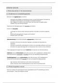
• Through cumulative distribution (reader p.7):
- Put findings in percentages
- Difference measure Δ = max Δ cp (which is where the curve is
vertically the most different → green arrow)
Δ > 30 is deemed large
• Effect size D (p. 13): difference bewteen centers relative to
distribution = with
2
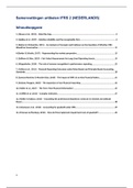
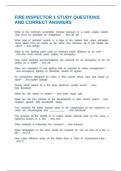
, Medians and quartiles (p. 8)
(These are alternatives in case of ordinal measures/
skewed distribution)
• Median: the ‘middle’ number (at 50%)
• Quartiles: at 25%, 50% and 75% → the boxplot
represents these values
• Useful for representing skewness and comparing
distributions
• Outlier (extremely high or low score): if the
whisker is longer than 1,5 times the lengths of the
box or z> 3
Lecture 3: explained variation
Variation analysis (p. 35)
• Total variation = SSd =
d can be calculated by the distance between each y-score and the overall mean
• Explained variation = SSg =
g is the deviation of the group mean from the general mean. To obtain SSg, square g and
multiply it by the group size and sum.
• Residual variation = SSe =
e is the deviation from group means for each y-score
• SSd = SSg + SSe
Eta2 = proportion of explained varation (p. 36)
• Eta2 = SSg/ SSd → see reader appendix 4: effect sizes
• It is the relative reduction of prediction error = proportion of variation in Y explained by X
• In case of two groups: eta2 = D2 / (4 + D2)
Linear regression (p. 38)
• A hypothetical, linear relationship between two variables and a way of predicting the value
of one variable from another
• It is a straight, linear line so the formula is:
B0 = intercept (value of Y when X = 0)
B = regression coefficient =
In SPSS, these can be found in the column ‘Unstandardized B’, the number next to (Constant)
is b0 and the one next to the variable is b
Testing the model (p. 39)
• Deviation observation = SSd : (deviation each y-score from the mean)
• Explained part = SSl : (deviation regression line from the mean)
3
Content
Part 1:
Lecture 1: intro ........................................................................................................................................ 2
Lecture 2: descriptive statistics ............................................................................................................... 2
Lecture 3: explained variation ................................................................................................................. 3
Lecture 4: theory of estimates and testing ............................................................................................. 4
Lecture 5: comparing two groups ........................................................................................................... 5
Lecture 6: comparing more groups ......................................................................................................... 7
Lecture 7: ANOVA with controls.............................................................................................................. 8
Part 2:
Lecture 9: association interval and ordinal variables .............................................................................. 9
Lecture 10: linear regression part 1 ...................................................................................................... 11
Lecture 11: linear regression part 2 ...................................................................................................... 13
Lecture 12: association nominal variables ............................................................................................ 15
Lecture 13: logistic regression ............................................................................................................... 17
Lecture 14: factor analysis..................................................................................................................... 18
1
,Part 1
Lecture 1: intro
Statistical toolbox
• (Arithmetic) mean =
• Dispersion = deviation of the individual scores from the mean = dev=
• Variance (a measure of dispersion of data):
SS = sum of squares = the sum of squared deviations
df = degrees of freedom (n-1 if sample)
Variance =
• Standard deviation = square root of the variance =
Lecture 2: descriptive statistics
Statistical techniques
• Descriptive statistics: describes/ summarize data in tables, graphs and metrics, and draw
conclusions regarding similarities and differences.
• Inductive statistics: can you generalize your findings to the population? So here, we look at if
the observed difference is more than a coincidence (statistically significant) and for example
what the estimated size of the difference between the populations is.
Levels of measurement
• Nominal: categorical variables that cannot be ordered (e.g. gender, sector)
• Ordinal: also categorical, but can be ordered (e.g. likert scale, Beaufort scale)
• Interval/ ratio: similar intervals on the scale indicate similar differences (e.g. weight (kg),
distance (m)). In SPSS this is named ‘scale’.
Metrics to express the amount of difference
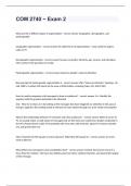
• Through cumulative distribution (reader p.7):
- Put findings in percentages
- Difference measure Δ = max Δ cp (which is where the curve is
vertically the most different → green arrow)
Δ > 30 is deemed large
• Effect size D (p. 13): difference bewteen centers relative to
distribution = with
2
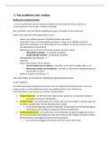
, Medians and quartiles (p. 8)
(These are alternatives in case of ordinal measures/
skewed distribution)
• Median: the ‘middle’ number (at 50%)
• Quartiles: at 25%, 50% and 75% → the boxplot
represents these values
• Useful for representing skewness and comparing
distributions
• Outlier (extremely high or low score): if the
whisker is longer than 1,5 times the lengths of the
box or z> 3
Lecture 3: explained variation
Variation analysis (p. 35)
• Total variation = SSd =
d can be calculated by the distance between each y-score and the overall mean
• Explained variation = SSg =
g is the deviation of the group mean from the general mean. To obtain SSg, square g and
multiply it by the group size and sum.
• Residual variation = SSe =
e is the deviation from group means for each y-score
• SSd = SSg + SSe
Eta2 = proportion of explained varation (p. 36)
• Eta2 = SSg/ SSd → see reader appendix 4: effect sizes
• It is the relative reduction of prediction error = proportion of variation in Y explained by X
• In case of two groups: eta2 = D2 / (4 + D2)
Linear regression (p. 38)
• A hypothetical, linear relationship between two variables and a way of predicting the value
of one variable from another
• It is a straight, linear line so the formula is:
B0 = intercept (value of Y when X = 0)
B = regression coefficient =
In SPSS, these can be found in the column ‘Unstandardized B’, the number next to (Constant)
is b0 and the one next to the variable is b
Testing the model (p. 39)
• Deviation observation = SSd : (deviation each y-score from the mean)
• Explained part = SSl : (deviation regression line from the mean)
3