Univariate linear time series
Time serie is a sequential set of observations on variable x, where t represents time Exa =..., Xe-2 ,
Xe ,
Xe ,
Xe +, Xe +, ...
Financial returns
-
One-period (simple) return PA Pe DA Pt-1 Pt Pt-1 DE
note
PA
-
+
-
- - 1
regular (if dividends are included
: RE =
Pt-1 Rt =
Pt -1 =
Pe -
1
+
Pt -1
) RE
returns
log-return =log) Rt) leg (p) :
log -log Pr , +
= =
pr -pe
= Pr =
spe Pt
price
-
Multi-period return (sum of one-period returns), use log-returns k - 1
dividens
De
re[k] =
pt
-
pe m
=
(pt -
pt
1) -
(pt ps k)
- =
ra +
(pt 1
-
pe
-z) +
(pec -
pe
-b) =
ra + re + ...
grej
#
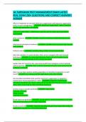
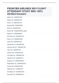
Using these concepts of time series and financial returns, we get financial time series
example
Prices Log of prices Log of return
properties financial time series
-
stationarity
strict stationarity: distribution of (xh + 1,
, . . .,
Xer +
1) does not depend on t for any integers Et , ....
Ab and t
distribution does not change when we shift, hence change t
7
weak stationarity
8
constant mean, independent of time: E(xt) M =
O
constant variance, independent of time: Var(xe) G =
El(x m)(x )]
constant autocovariance, independent of time: (x
e)
O
for( j
: - -
=
,
-
autocorrelation function ACF: pl =
core (xt ,
xx e) =
Var(xe) =
yo
D E(ae) Var(ae) Cov(at are)
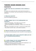
example stationary process, White Noise: = 0
,
=
8, ,
=
o
models
d
Linear process: m j +jatj m Xt =
+ = + Nodt + 4 , at - ....
Pit
stationary with mean M , variance z4, and ACF Al 204j
7 =
Wold's decomposition theory states that any stationary proces [xe] can be written as sum of linear and
deterministic processes Ewa]
We could also at a lag operator B, defined by Bxt =
XA -
, hence Baxt =
Xe b -
I
, N
Then we could write the linear process as xt =
m
+ x(B) at =
m
+ 4oat + 4 , at - ...
+ That - b
- +(B) =
j4 B ,
8
Autoregressive process
· AR( ) ,
:
xt =
00 + Ext -1 + at
①o Ga
7
stationary if 10 14 , then E(x) A Var(xz) -0 ,
yo
= =
m
=
. =
1 -
, 1
proof 00 Xt = + 6 , Xt -
1 + at
(1 -
d, B) xt =
00 + at
x =
,)1 qB)" (d at)
-
+ =
j(q B)" (4,
+ a) =
Tod, (0 +
atj)
-
d(B) =
1 - d B ,
=
0
&
AR( ) 4
5
ACF ,
stationary 1
is linear process with exponentially decaying weights =
6 ,
, we find =
pe
=
0
AR(p)
·
:
xt = do + d , xt -
1 + +
6pxt -
p
+ at
example
...
Et
ye
0
3yt +
=
0
1yt
. - + .
-
2
>
stationary if all zj lie outside unit circle: ye
-
0 .
3yt -
1
-
0 .
1yt 2
=
Et
xt- t
proof X- ·
,
(1 -
0 .
3) -
o .,
(2) ye =
Es
↓ (2) 122
for =
1 -
0 32.
-
0 .
= 0 2 = -
522 = 2
((z) =
1 -
0 , 2 ....
-
pzP = 0 #
as both lie outside unit circle, stationary
&
ACF can not be determined, but we can use partial autocorrelation function (PACF), for
AR(p), the PACF has cut-off point at l p =
Q
Moving Average model
·
MA(1) :
x =
20 + at -
G at -1
,
7
stationary for all parameter values with M ja) +i)
jo er =
=
1 +
,
-- for hence ACF is cut-off at l peo
>
,
p 1
. =
,
>
invertible if 18 14 .
, a model is invertible if it can be expressed as AR(n)
proof XA =
at + fat -
1
at =
xx
-
G , at -
1
=
Xt - 0(xt - - at z) =... =
x -
Ext + + 0xx 2 - 83x 3 + ...
D
( f)" AR(g) 101
= -
i =
-
+ a =
only works as
>
PACF decays exponentially
MA(q)
·
at-Gat- . . .
xt co
gatg
-
: = +
>
ACF has cut-off point at l g =
invertible if all roots zj lie outside unit circle: Fiat -
at
gatq
7
Xt e0
-
=
+ -
-...
xe =
e +
1) -
f B ,
-
...
fqB) at ,
Xe = e + (B) at
6(z) =
1
-
12 ...
-
gz = o
&
PACF decays exponentially
, &
Mixed autoregressive-moving average model
ARMA(p g)
·
d dx ApX - G,
,
EqAq :
xt = + + + ... +
-p
+ at ....
①o O(z)
b(z) y(B)at (2)
stationary if all roots of
7
lie outside unit circle, implying xx =
m
+
,
m
=
0)) ,
=
q(z)
((z)
3
invertible if all roots of f(z) lie outside unit circle, yielding # (B) x1 = co + at
,
20 =
0(1) ,
(2) =
f(z)
7
ACF decays exponentially
>
PACF decays exponentially
&
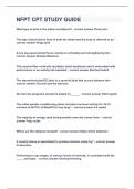
ARMA(p 1)
To avoid identification problems, reduce model to -1 ,
g
-
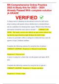
AR(p) MA(g) ARMA(p ,
g)
AlF deceases geometrically
,
pl I 1
for large l
11
decreases geometrically 0 for 2q
PACF ,
60 I I deceases geometrically
for large l
0 for expo decreases geometrically
8
Integrated processes: many time series are non-stationary, but may have stationary first differences
X-X
example is non-stationary, but is stationary, now 1( ) Xe -
is integrated of order d ( = ) if
Xt =
Xt -
1 + Et ,
hence
7 Xt
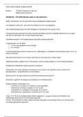
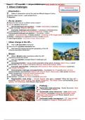
stationary vs integrated processes
now we applicate this to the ARMA(p g) model: ,
:
Xt =
00 + b , Xt -
1 + ...
+
6pXt p
+ at -
, at - - ...
-
Agat-q :
ApXt 0 Eat
xx d , Xt = + at ....
OgAq
-
p
-
-
....
((B)xt = 6 f(B) at
when this is non-stationary we could use differences
+
( (B)axx =
00 + f(B) at
(with roots ↓ (B) and &(B) outside unit circle)
>
autoregressive-integrated-moving average, ARIMA(p d g) , ,
example random walk (with drift if MF0 ) : Xt =
M
+ Xt -
1 + at
E(x0) Var(x)
xo
Mt aj this is non-stationary as Mt Var(xe) ot
= + = +
m
+ = +
,
but we can integrate to make stationary: AXt =
M
+ at
Suppose we have a time series, how do we then select the appropriate ARIMA model?
>
Box-Jenkins procedure: consists of servers steps
1
Identification /model selection: make initial guess of p, d and q, based on graphs and sample ACF and PACF
L
remember
sample ACF je jo
je i (x x)(xx z)
(xe )
Leung-Box Q-statistic
test
Hope
=
Haiplo Q(m) T(T 2) x (m)
=
+,
-
-
*
e -
3 =
0
,
=
+
<
~
sample PACF Ee] : obtain with OLS on Xt =
00 ,
2 +
d1 ,
2xt - ...
+ PhlXt 1 + elt
:
...
& l
or 2 .
l L
: i
= ...
I
Fre
Time serie is a sequential set of observations on variable x, where t represents time Exa =..., Xe-2 ,
Xe ,
Xe ,
Xe +, Xe +, ...
Financial returns
-
One-period (simple) return PA Pe DA Pt-1 Pt Pt-1 DE
note
PA
-
+
-
- - 1
regular (if dividends are included
: RE =
Pt-1 Rt =
Pt -1 =
Pe -
1
+
Pt -1
) RE
returns
log-return =log) Rt) leg (p) :
log -log Pr , +
= =
pr -pe
= Pr =
spe Pt
price
-
Multi-period return (sum of one-period returns), use log-returns k - 1
dividens
De
re[k] =
pt
-
pe m
=
(pt -
pt
1) -
(pt ps k)
- =
ra +
(pt 1
-
pe
-z) +
(pec -
pe
-b) =
ra + re + ...
grej
#
Using these concepts of time series and financial returns, we get financial time series
example
Prices Log of prices Log of return
properties financial time series
-
stationarity
strict stationarity: distribution of (xh + 1,
, . . .,
Xer +
1) does not depend on t for any integers Et , ....
Ab and t
distribution does not change when we shift, hence change t
7
weak stationarity
8
constant mean, independent of time: E(xt) M =
O
constant variance, independent of time: Var(xe) G =
El(x m)(x )]
constant autocovariance, independent of time: (x
e)
O
for( j
: - -
=
,
-
autocorrelation function ACF: pl =
core (xt ,
xx e) =
Var(xe) =
yo
D E(ae) Var(ae) Cov(at are)
example stationary process, White Noise: = 0
,
=
8, ,
=
o
models
d
Linear process: m j +jatj m Xt =
+ = + Nodt + 4 , at - ....
Pit
stationary with mean M , variance z4, and ACF Al 204j
7 =
Wold's decomposition theory states that any stationary proces [xe] can be written as sum of linear and
deterministic processes Ewa]
We could also at a lag operator B, defined by Bxt =
XA -
, hence Baxt =
Xe b -
I
, N
Then we could write the linear process as xt =
m
+ x(B) at =
m
+ 4oat + 4 , at - ...
+ That - b
- +(B) =
j4 B ,
8
Autoregressive process
· AR( ) ,
:
xt =
00 + Ext -1 + at
①o Ga
7
stationary if 10 14 , then E(x) A Var(xz) -0 ,
yo
= =
m
=
. =
1 -
, 1
proof 00 Xt = + 6 , Xt -
1 + at
(1 -
d, B) xt =
00 + at
x =
,)1 qB)" (d at)
-
+ =
j(q B)" (4,
+ a) =
Tod, (0 +
atj)
-
d(B) =
1 - d B ,
=
0
&
AR( ) 4
5
ACF ,
stationary 1
is linear process with exponentially decaying weights =
6 ,
, we find =
pe
=
0
AR(p)
·
:
xt = do + d , xt -
1 + +
6pxt -
p
+ at
example
...
Et
ye
0
3yt +
=
0
1yt
. - + .
-
2
>
stationary if all zj lie outside unit circle: ye
-
0 .
3yt -
1
-
0 .
1yt 2
=
Et
xt- t
proof X- ·
,
(1 -
0 .
3) -
o .,
(2) ye =
Es
↓ (2) 122
for =
1 -
0 32.
-
0 .
= 0 2 = -
522 = 2
((z) =
1 -
0 , 2 ....
-
pzP = 0 #
as both lie outside unit circle, stationary
&
ACF can not be determined, but we can use partial autocorrelation function (PACF), for
AR(p), the PACF has cut-off point at l p =
Q
Moving Average model
·
MA(1) :
x =
20 + at -
G at -1
,
7
stationary for all parameter values with M ja) +i)
jo er =
=
1 +
,
-- for hence ACF is cut-off at l peo
>
,
p 1
. =
,
>
invertible if 18 14 .
, a model is invertible if it can be expressed as AR(n)
proof XA =
at + fat -
1
at =
xx
-
G , at -
1
=
Xt - 0(xt - - at z) =... =
x -
Ext + + 0xx 2 - 83x 3 + ...
D
( f)" AR(g) 101
= -
i =
-
+ a =
only works as
>
PACF decays exponentially
MA(q)
·
at-Gat- . . .
xt co
gatg
-
: = +
>
ACF has cut-off point at l g =
invertible if all roots zj lie outside unit circle: Fiat -
at
gatq
7
Xt e0
-
=
+ -
-...
xe =
e +
1) -
f B ,
-
...
fqB) at ,
Xe = e + (B) at
6(z) =
1
-
12 ...
-
gz = o
&
PACF decays exponentially
, &
Mixed autoregressive-moving average model
ARMA(p g)
·
d dx ApX - G,
,
EqAq :
xt = + + + ... +
-p
+ at ....
①o O(z)
b(z) y(B)at (2)
stationary if all roots of
7
lie outside unit circle, implying xx =
m
+
,
m
=
0)) ,
=
q(z)
((z)
3
invertible if all roots of f(z) lie outside unit circle, yielding # (B) x1 = co + at
,
20 =
0(1) ,
(2) =
f(z)
7
ACF decays exponentially
>
PACF decays exponentially
&
ARMA(p 1)
To avoid identification problems, reduce model to -1 ,
g
-
AR(p) MA(g) ARMA(p ,
g)
AlF deceases geometrically
,
pl I 1
for large l
11
decreases geometrically 0 for 2q
PACF ,
60 I I deceases geometrically
for large l
0 for expo decreases geometrically
8
Integrated processes: many time series are non-stationary, but may have stationary first differences
X-X
example is non-stationary, but is stationary, now 1( ) Xe -
is integrated of order d ( = ) if
Xt =
Xt -
1 + Et ,
hence
7 Xt
stationary vs integrated processes
now we applicate this to the ARMA(p g) model: ,
:
Xt =
00 + b , Xt -
1 + ...
+
6pXt p
+ at -
, at - - ...
-
Agat-q :
ApXt 0 Eat
xx d , Xt = + at ....
OgAq
-
p
-
-
....
((B)xt = 6 f(B) at
when this is non-stationary we could use differences
+
( (B)axx =
00 + f(B) at
(with roots ↓ (B) and &(B) outside unit circle)
>
autoregressive-integrated-moving average, ARIMA(p d g) , ,
example random walk (with drift if MF0 ) : Xt =
M
+ Xt -
1 + at
E(x0) Var(x)
xo
Mt aj this is non-stationary as Mt Var(xe) ot
= + = +
m
+ = +
,
but we can integrate to make stationary: AXt =
M
+ at
Suppose we have a time series, how do we then select the appropriate ARIMA model?
>
Box-Jenkins procedure: consists of servers steps
1
Identification /model selection: make initial guess of p, d and q, based on graphs and sample ACF and PACF
L
remember
sample ACF je jo
je i (x x)(xx z)
(xe )
Leung-Box Q-statistic
test
Hope
=
Haiplo Q(m) T(T 2) x (m)
=
+,
-
-
*
e -
3 =
0
,
=
+
<
~
sample PACF Ee] : obtain with OLS on Xt =
00 ,
2 +
d1 ,
2xt - ...
+ PhlXt 1 + elt
:
...
& l
or 2 .
l L
: i
= ...
I
Fre