Supply Chain Modelling
Msc Supply Chain Management
Tilburg University
Summary of all models
Model Chapter 4 – Demand Shock Dynamics: Cyclicality
Model Chapter 5 – In Praise of Lies? / ASML
Model Chapter 6 – Relevance Assumed / Interpolis
Model Chapter 7 – The Boiled Frog
Model Chapter 8 – Pilot Error / Airbus
Model Chapter 9 – The Service Quality Cascade / KPN
Model Chapter 10 – Travail, Transparency & Trust / Philips
Model Chapter 11 – Virtuous & Vicious Cycles in ERP Implementation
Model Chapter 12 – Collaborative KPI’s
For each model:
- Theoretical background
- The key feedback loops
- Explanation of every area (block) of the model in Silico
- Explained what goes wrong in the Base Case (Historically)
- Solutions to improve the model: what works and what not?
,Model Chapter 4 – Demand Shock Dynamics: Cyclicality
Background: 2 problems often occur after each other:
1. Demand goes up, but there is not directly enough capacity to meet demand → lost sales
2. Demand goes down, capacity is not timely reduced → low capacity utilization,
high inventory
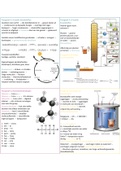
Key loops:
Balancing inventory loop: More orders → higher order backlog → more production → more finished
goods → more shipments → lower order backlog
Balancing capacity loop: Higher order backlog → higher desired capacity → more capacity → more
shipments → lower order backlog
The second balancing loop has the same result as the first one, but it takes way more time.
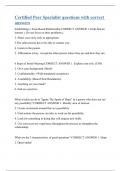
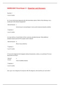
Model build-up:
Order handling: We have new orders coming in. These go into order backlog because not all orders
can be fulfilled immediately. The order fulfilment rate is the speed at which orders are delivered. This
is either the order backlog (you can’t deliver more than you have) or the shipments (you don’t ship
more than the demand is). It takes time to ship all your goods, that is expressed in the delivery delay.
Delivery performance is a measure on if the company meets their delivery targets. Lastly, the
company can limit how busy they want to be with orders by setting a max workload.
Production process: We see the logical process: production starts → work in progress → products
are finished → products are shipped. How long it takes to finish an order is expressed in the
production cycle time.
Furthermore, it is taken into account that finished goods are worth more than work in progress goods
when calculating inventory.
Capacity management process: The smoothed desired capacity is a function of what happens in the
production process. If there is a high order backlog and a high workload, there is a demand for a
higher capacity. But if you want more capacity, this cannot be done immediately. It takes time to
adjust capacity (capacity change rate).
Production planning: How much you want to produce depends on how many orders there are placed
and your current inventory level (desired production from orders and stock). Companies forecast the
demand to estimate how many products will be ordered in the future. But it also depends on your
capacity (desired production from capacity) because it is very costly to have a low capacity
utilization. In other words, if you have many machines you want them to be running.
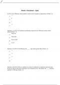
,What happened in Base Case?:
Halfway the year, we see a peak in demand for the semiconductors. Thereafter, we see that demand
drops. The company was unable to scale production up when demand increased. When the capacity
available was high enough, the demand was already much lower. We see that at this point inventory
increases because we produce more, but don’t sell it.
Proposed policies:
We know from theory that when there are at least two negative feedback loops with some delay in
it, oscillation occurs (= repeated fluctuation).
One way of solving this is to make capacity fixed (set SW Flex Cap = 0). This shows that the oscillation
is caused by the capacity loop in this case.
Operational improvements: Saying ‘no’ to customers. You can do this by limiting the amount of
orders by decreasing the max workload (f.e. from 4 to 2). Though in theory this could work (the
oscillation becomes less in this scenario), you don’t want to do it. Simply because you don’t like
saying ‘no’ to your customers.
Tactical improvements: Decreasing the production planning delay (f.e. from 6 to 1) and cap planning
adj delay (also to 1) does not solve the oscillation. This shows that quickening both the production
and capacity delays does not really solve the problem, but there is some improvement. Your
response becomes quicker but this makes your organization also more nervous.
Strategic improvements: Here we look at changing capacity. This is at strategic level, because it is
very costly and time-consuming. But what if we can adjust capacity quicker? If we reduce the
capacity acquisition delay (f.e. from 36 periods to 24) we see that this reduces the oscillation and we
are also better able to meet demand. This may be a good solution, but the question is if this is
possible. A downside is that it again makes the organization more nervous.
, Model Chapter 5 – ASML
Background: a very high peak in demand in the year 2000, resulting in more orders placed than the
number of actual shipments. Not everyone gets what they demanded. So, companies start to order
more than they really need in order to receive what they actually need: bullwhip effect.
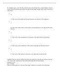
Vicious cycle: Companies order more → more capacity shortages → longer lead times → more
demand inflation → even more orders → etc.
After some time, customers have received what they needed and the demand for new orders drops
heavily.
Problems: You would like to have more capacity soon, but you can’t
You would like to control demand, but you can’t
→ In order to stop the vicious cycle, you can try to not be too transparent in your supply chain
problems → don’t let your customers know that you have shortages → but this does not work
enough.
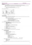
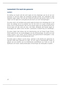
Model build-up:
- Order flow at OEM: Order backlog: Placed orders that aren’t delivered yet. Products in order
backlog can either be shipped or cancelled. The number of shipments is the lowest value between
capacity (you can’t ship more than you produce) and the desired shipments (you are not shipping
more than the customers demand).
Formula for lead time is little’s law.
- Order management at customer base: You can see the peak in real customer demand. If customers
expect a longer lead time, they will order more then they need (shortage gaming multiplier). This will
increase demand, until cum demand is lower than cum shipments (so when the customers have what
they want), then you see a sudden drop in demand. Then the bubble bursts.
- Lead time visibility for customer base: The communicated lead time is determined by the actual
lead time and a change in comm lead time. That is, the company does not immediately tell customers
about a change in lead time. The time they wait is the LT communication delay.
But, the LT that customers hold on to is not only what is communicated to them, but also what they
actually experience. An important indicator for that is the delivery reliability. This reliability is
determined by workload (the busier, the less reliable).
- Capacity management in supply base: If there is a change in perceived demand, then there comes a
new desired capacity. Then you change capacity to come to a new capacity, but this takes time (time
to adjust capacity). So, the capacity has the same curve as the demand since you want to adjust
capacity to the demand.
Msc Supply Chain Management
Tilburg University
Summary of all models
Model Chapter 4 – Demand Shock Dynamics: Cyclicality
Model Chapter 5 – In Praise of Lies? / ASML
Model Chapter 6 – Relevance Assumed / Interpolis
Model Chapter 7 – The Boiled Frog
Model Chapter 8 – Pilot Error / Airbus
Model Chapter 9 – The Service Quality Cascade / KPN
Model Chapter 10 – Travail, Transparency & Trust / Philips
Model Chapter 11 – Virtuous & Vicious Cycles in ERP Implementation
Model Chapter 12 – Collaborative KPI’s
For each model:
- Theoretical background
- The key feedback loops
- Explanation of every area (block) of the model in Silico
- Explained what goes wrong in the Base Case (Historically)
- Solutions to improve the model: what works and what not?
,Model Chapter 4 – Demand Shock Dynamics: Cyclicality
Background: 2 problems often occur after each other:
1. Demand goes up, but there is not directly enough capacity to meet demand → lost sales
2. Demand goes down, capacity is not timely reduced → low capacity utilization,
high inventory
Key loops:
Balancing inventory loop: More orders → higher order backlog → more production → more finished
goods → more shipments → lower order backlog
Balancing capacity loop: Higher order backlog → higher desired capacity → more capacity → more
shipments → lower order backlog
The second balancing loop has the same result as the first one, but it takes way more time.
Model build-up:
Order handling: We have new orders coming in. These go into order backlog because not all orders
can be fulfilled immediately. The order fulfilment rate is the speed at which orders are delivered. This
is either the order backlog (you can’t deliver more than you have) or the shipments (you don’t ship
more than the demand is). It takes time to ship all your goods, that is expressed in the delivery delay.
Delivery performance is a measure on if the company meets their delivery targets. Lastly, the
company can limit how busy they want to be with orders by setting a max workload.
Production process: We see the logical process: production starts → work in progress → products
are finished → products are shipped. How long it takes to finish an order is expressed in the
production cycle time.
Furthermore, it is taken into account that finished goods are worth more than work in progress goods
when calculating inventory.
Capacity management process: The smoothed desired capacity is a function of what happens in the
production process. If there is a high order backlog and a high workload, there is a demand for a
higher capacity. But if you want more capacity, this cannot be done immediately. It takes time to
adjust capacity (capacity change rate).
Production planning: How much you want to produce depends on how many orders there are placed
and your current inventory level (desired production from orders and stock). Companies forecast the
demand to estimate how many products will be ordered in the future. But it also depends on your
capacity (desired production from capacity) because it is very costly to have a low capacity
utilization. In other words, if you have many machines you want them to be running.
,What happened in Base Case?:
Halfway the year, we see a peak in demand for the semiconductors. Thereafter, we see that demand
drops. The company was unable to scale production up when demand increased. When the capacity
available was high enough, the demand was already much lower. We see that at this point inventory
increases because we produce more, but don’t sell it.
Proposed policies:
We know from theory that when there are at least two negative feedback loops with some delay in
it, oscillation occurs (= repeated fluctuation).
One way of solving this is to make capacity fixed (set SW Flex Cap = 0). This shows that the oscillation
is caused by the capacity loop in this case.
Operational improvements: Saying ‘no’ to customers. You can do this by limiting the amount of
orders by decreasing the max workload (f.e. from 4 to 2). Though in theory this could work (the
oscillation becomes less in this scenario), you don’t want to do it. Simply because you don’t like
saying ‘no’ to your customers.
Tactical improvements: Decreasing the production planning delay (f.e. from 6 to 1) and cap planning
adj delay (also to 1) does not solve the oscillation. This shows that quickening both the production
and capacity delays does not really solve the problem, but there is some improvement. Your
response becomes quicker but this makes your organization also more nervous.
Strategic improvements: Here we look at changing capacity. This is at strategic level, because it is
very costly and time-consuming. But what if we can adjust capacity quicker? If we reduce the
capacity acquisition delay (f.e. from 36 periods to 24) we see that this reduces the oscillation and we
are also better able to meet demand. This may be a good solution, but the question is if this is
possible. A downside is that it again makes the organization more nervous.
, Model Chapter 5 – ASML
Background: a very high peak in demand in the year 2000, resulting in more orders placed than the
number of actual shipments. Not everyone gets what they demanded. So, companies start to order
more than they really need in order to receive what they actually need: bullwhip effect.
Vicious cycle: Companies order more → more capacity shortages → longer lead times → more
demand inflation → even more orders → etc.
After some time, customers have received what they needed and the demand for new orders drops
heavily.
Problems: You would like to have more capacity soon, but you can’t
You would like to control demand, but you can’t
→ In order to stop the vicious cycle, you can try to not be too transparent in your supply chain
problems → don’t let your customers know that you have shortages → but this does not work
enough.
Model build-up:
- Order flow at OEM: Order backlog: Placed orders that aren’t delivered yet. Products in order
backlog can either be shipped or cancelled. The number of shipments is the lowest value between
capacity (you can’t ship more than you produce) and the desired shipments (you are not shipping
more than the customers demand).
Formula for lead time is little’s law.
- Order management at customer base: You can see the peak in real customer demand. If customers
expect a longer lead time, they will order more then they need (shortage gaming multiplier). This will
increase demand, until cum demand is lower than cum shipments (so when the customers have what
they want), then you see a sudden drop in demand. Then the bubble bursts.
- Lead time visibility for customer base: The communicated lead time is determined by the actual
lead time and a change in comm lead time. That is, the company does not immediately tell customers
about a change in lead time. The time they wait is the LT communication delay.
But, the LT that customers hold on to is not only what is communicated to them, but also what they
actually experience. An important indicator for that is the delivery reliability. This reliability is
determined by workload (the busier, the less reliable).
- Capacity management in supply base: If there is a change in perceived demand, then there comes a
new desired capacity. Then you change capacity to come to a new capacity, but this takes time (time
to adjust capacity). So, the capacity has the same curve as the demand since you want to adjust
capacity to the demand.