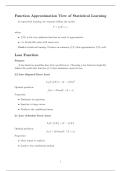
In supervised learning, the response follows the model:
Y = f (X) + ε,
where:
• f (X) is the true unknown function we want to approximate.
• ε is irreducible noise with mean zero.
Goal of statistical learning: Produce an estimator fˆ(X) that approximates f (X) well.
Loss Function
Purpose
A loss function quantifies how bad a prediction is. Choosing a loss function implicitly
defines the prediction function f (x) that minimizes expected loss.
L2 Loss (Squared Error Loss)
L2 (Y, f (X)) = (Y − f (X))2
Optimal predictor:
f (x) = M ean[Y | X = x]
Properties:
• Dominant in regression.
• Sensitive to large errors.
• Produces the conditional mean.
L1 Loss (Absolute Error Loss)
L1 (Y, f (X)) = |Y − f (X)|
Optimal predictor:
f (x) = M edian(Y | X = x)
Properties:
• More robust to outliers.
• Leads to the conditional median.
1
,Loss 0–1 (Classification Loss)
L0−1 (Y, f (X)) = 1[Y ̸= f (X)]
Optimal predictor:
f (x) = M ode(Y | X = x)
Properties:
• Used in classification.
• Minimizing 0–1 loss yields the Bayes classifier.
Bias Variance Trade-off
Under L2 loss, expected test error decomposes into:
E[(Y − fˆ(X))2 ] = Var[fˆ(X)] + (Bias[fˆ(X)])2 + Var[ε]
| {z } | {z } | {z } | {z }
T estError V ariance SquaredBias IrreducibleError
Bias
• Error that occurs when a model is too simple to capture the true patterns in the
data
• High bias: The model oversimplifies → misses patterns and underfits the
data.
• Low bias: The model captures patterns well and is closer to the true values
→ Overfits
Variance
• How much a model’s predictions change when it’s trained on different data.
• High variance: The model is too sensitive to small changes ⇒ overfitting
• Low variance: The model is more stable but might miss some patterns →
Underfits
Reducible Error
E[(f (X) − fˆ(X))2 ] = Var[fˆ(X)] + (Bias[fˆ(X)])2
| {z } | {z } | {z }
ReducibleError V ariance SquaredBias
• Origin: Inability to perfectly estimate the true function f(X)
• Reducible error = bias² + variance
• Reason: Use an approximation (a model) instead of the true function
2
, • How to reduce bias:
– Use more complex models
– Using more relevant features
– Reduce regularization to allow the model more flexibility in fitting
• How to reduce variance:
– Simplify the model
– Increase training data
– Apply regularization to constrain model complexity
– Use ensemble methods
Irreducible Error
• Origin: Random noise term ε
• Even if we know the true function f (X) → ε still cause variability in Y
• Reason: ε is independent of X
Trade-off
• Increasing model flexibility decreases bias but increases variance.
• Goal: choose a model complexity (λ, number of features, neighbors k, etc.) that
minimizes test error, not training error.
Training Error vs Test Error & Generalization Error
Training Error
• Computed on data used to fit the model.
• Typically underestimates true error.
• Flexible models can make training error nearly zero.
Test Error
• Error on previously unseen data.
• Used to estimate real-world performance.
Generalization Error
• True population-level predictive error.
• Not observable directly.
• Test error is an estimate of generalization error.
Training error is not reliable because the model is optimized to minimize it.
3

