Macroeconomics I: Summary
Tim Eijkenaar
May 2020
1
,Contents
1 GDP Accounting 4
1.1 GDP . . . . . . . . . . . . . . . . . . . . . . . . . . . . . . . . . . . . . . . . . . . . . 4
1.2 Expenditure components of GDP . . . . . . . . . . . . . . . . . . . . . . . . . . . . . 4
1.3 Price indexes . . . . . . . . . . . . . . . . . . . . . . . . . . . . . . . . . . . . . . . . 4
2 Unemployment 5
2.1 Measuring joblessness . . . . . . . . . . . . . . . . . . . . . . . . . . . . . . . . . . . 5
2.2 The natural rate of unemployment . . . . . . . . . . . . . . . . . . . . . . . . . . . . 5
3 Economic growth 6
3.1 Production function . . . . . . . . . . . . . . . . . . . . . . . . . . . . . . . . . . . . 6
3.2 Cobb-Douglas production function . . . . . . . . . . . . . . . . . . . . . . . . . . . . 7
4 Solow growth model 8
4.1 The production function . . . . . . . . . . . . . . . . . . . . . . . . . . . . . . . . . . 8
4.2 Steady state level of capital . . . . . . . . . . . . . . . . . . . . . . . . . . . . . . . . 9
4.3 Golden rule level of capital . . . . . . . . . . . . . . . . . . . . . . . . . . . . . . . . 10
4.4 The effect of efficiency and population growth . . . . . . . . . . . . . . . . . . . . . . 12
5 Money and banking 13
5.1 Money . . . . . . . . . . . . . . . . . . . . . . . . . . . . . . . . . . . . . . . . . . . . 13
5.2 The quantity equation . . . . . . . . . . . . . . . . . . . . . . . . . . . . . . . . . . . 13
5.3 The demand for money . . . . . . . . . . . . . . . . . . . . . . . . . . . . . . . . . . 14
5.4 The Fisher effect . . . . . . . . . . . . . . . . . . . . . . . . . . . . . . . . . . . . . . 14
5.5 The cost of holding money . . . . . . . . . . . . . . . . . . . . . . . . . . . . . . . . . 15
5.6 Exchange rates . . . . . . . . . . . . . . . . . . . . . . . . . . . . . . . . . . . . . . . 15
6 Aggregate demand and supply 16
6.1 Aggregate demand . . . . . . . . . . . . . . . . . . . . . . . . . . . . . . . . . . . . . 16
6.2 Aggregate supply . . . . . . . . . . . . . . . . . . . . . . . . . . . . . . . . . . . . . . 17
6.3 Aggregate supply = aggregate demand . . . . . . . . . . . . . . . . . . . . . . . . . . 17
6.4 Shocks . . . . . . . . . . . . . . . . . . . . . . . . . . . . . . . . . . . . . . . . . . . . 18
7 IS-LM Model 19
7.1 IS-Curve . . . . . . . . . . . . . . . . . . . . . . . . . . . . . . . . . . . . . . . . . . 19
7.2 Shifting the IS-curve . . . . . . . . . . . . . . . . . . . . . . . . . . . . . . . . . . . . 20
7.3 LM -Curve . . . . . . . . . . . . . . . . . . . . . . . . . . . . . . . . . . . . . . . . . . 21
7.4 Shifting the LM -curve . . . . . . . . . . . . . . . . . . . . . . . . . . . . . . . . . . . 21
7.5 Equilibrium analysis . . . . . . . . . . . . . . . . . . . . . . . . . . . . . . . . . . . . 22
7.6 Multipliers . . . . . . . . . . . . . . . . . . . . . . . . . . . . . . . . . . . . . . . . . 23
8 Mundell-Fleming model 24
8.1 IS ∗ -curve . . . . . . . . . . . . . . . . . . . . . . . . . . . . . . . . . . . . . . . . . . 24
8.2 When do we shift the IS ∗ -curve? . . . . . . . . . . . . . . . . . . . . . . . . . . . . . 24
8.3 LM ∗ -curve . . . . . . . . . . . . . . . . . . . . . . . . . . . . . . . . . . . . . . . . . 25
2
, 8.4 When do we shift the LM ∗ curve? . . . . . . . . . . . . . . . . . . . . . . . . . . . . 25
8.5 Equilibrium analysis . . . . . . . . . . . . . . . . . . . . . . . . . . . . . . . . . . . . 26
8.6 Fixed exchange rates . . . . . . . . . . . . . . . . . . . . . . . . . . . . . . . . . . . . 27
8.7 Equilibrium analysis: e = e . . . . . . . . . . . . . . . . . . . . . . . . . . . . . . . . 27
9 Three models of aggregate supply 29
9.1 The sticky-price model . . . . . . . . . . . . . . . . . . . . . . . . . . . . . . . . . . . 29
9.2 The sticky-wage model . . . . . . . . . . . . . . . . . . . . . . . . . . . . . . . . . . . 30
9.3 Imperfect information model . . . . . . . . . . . . . . . . . . . . . . . . . . . . . . . 30
9.4 The new SRAS . . . . . . . . . . . . . . . . . . . . . . . . . . . . . . . . . . . . . . . 30
10 Phillips curve 31
3
,1 GDP Accounting
1.1 GDP
Let Qi,t denote the quantity of product i at year t and let Pi,t be the price of product i at year t.
Assume the chosen base year is t = 0. Then,
X
Real GDP at year t = Pi,0 ∗ Qi,t
i
X
Nominal GDP at year t = Pi,t ∗ Qi,t
i
1.2 Expenditure components of GDP
The four expenditure components of GDP are given by the following formula: Y = C + I + G + N X
Y = Output = Income = GDP
C = Consumption = C(Y − T )
I = Investment = I(r)
G = Government spending
N X = Net exports = N X(e)
Where we used the fact that output Y is a function of disposable income (Y − T ), investment I is
a function of the interest rate r and N X is a function of the exchange rate e.
We define:
Trade deficit = X − M = Exports − Imports
Capital inflow = −N X
Furthermore we have the following formulas where we assume a closed economy (N X = 0):
Private saving = Y − T − C
Public saving = T − G
Saving = S = (Y − T − C) + (T − G) = I
1.3 Price indexes
Both the Paasche price index and the Laspeyres price index reflect what is happening to the price
level in the economy. They are defined in the following way.
P
Nominal GDP at year t Pi,t ∗ Qi,t
Paasche price index = GDP Deflator = = Pi
Real GDP at year t i Pi,0 ∗ Qi,t
P
P i,t ∗ Qi,0
Laspeyres price index = CPI = P i
i P i,0 ∗ Q i,0
4
,2 Unemployment
2.1 Measuring joblessness
Each adult is placed into one of the following three categories:
1. Employed E
2. Unemployed U
3. Not in the labour force
We define
Labour force = Number of employed + Number of unemployed
Number of employed
Unemployment rate = ∗ 100%
Labour force
Labour force
Labour force participation rate = ∗ 100%
Adult population
2.2 The natural rate of unemployment
It is reasonable to assume that the labour force L is fixed. The unemployment rate is under this
assumption fully determined by the transition of individuals in the labour force. Let s denote the
rate of job separation and let f denote the rate of job finding. Then the number of people that lose
their job sE must be equal to the number of people that find a new job f U .
f U = sE
f U = s(L − U )
U 1
=
L 1 + f/s
Where we used the fact that E = L − U and did some basic algebra steps to derive the last formula.
5
,3 Economic growth
3.1 Production function
Output Y , or GDP, is a function of the amount of capital K and the amount of labour L.
That is, Y = F (K, L).
A production function has the property ’constant returns to scale’ if zY = F (zK, zL) for every real
number z.
The marginal product of labour M P L is the extra amount of output a firm gets given a unit change
in the amount of labour. That is, M P L is the partial derivative of F with respect to L:
∂F (K, L)
MPL =
∂L
Likewise, the marginal product of capital M P K is the change in the amount of output given a unit
change in the amount of capital:
∂F (K, L)
MPK =
∂K
The above gives us the following result: let P be the price of one single unit of output and let W
be the wage corresponding to one unit of labour. Then if we increase L by one unit:
∆Profit = ∆Revenues − ∆Cost
= MPL ∗ P − W
Intuitively, as long as ∆Profit > 0 we want to increase the amount of labour until ∆Profit = 0.
Therefore, every competitive firm will satisfy
∆Profit = ∆Revenues − ∆Cost
0 = MPL ∗ P − W
W
MPL =
P
We can do the same steps for the M P K. This will lead us to the following result:
R
MPK =
P
6
,3.2 Cobb-Douglas production function
Any production function of the form F (K, L) = A K α L1−α with A > 0 and 0 ≤ α ≤ 1 is called a
’Cobb-Douglas production function’.
Note that F has constant return to scale since
F (zK, zL) = A(zK)α (zL)1−α = AK α L1−α z α z 1−α = zA K α L1−α = zF (K, L)
Furthermore for every Cobb-Douglas production function it holds that
Y
M P L = (1 − α)AK α L−α = (1 − α)
L
Y
M P K = αAK α−1 L1−α = α
K
7
,4 Solow growth model
4.1 The production function
Recall that the production function is given by F (K, L). In the Solow growth model we assume
that F has constant return to scale: zF (K, L) = F (zK, zL). Furthermore, we want to analyse
all quantities in the economy relative to the size of the labour force. That means that we are not
interested in output Y itself, but in YL . We now rewrite Y = F (K, L) to know more about YL . We
use the fact that F has constant return to scale. Note that in this case z = L1 :
Y = F (K, L)
Y F (K, L)
=
L L
K L
= F( , )
L L
K
= F( , 1)
L
From now on, we denote every variable relative to the size of the labour force with just the small
letter of the variable:
Y K C
=y =k =c
L L L
We can now rewrite our production function. Note that we can simply forget about the variable ’1’
since it is a constant. We use f instead of F for convenience.
Y K
= F ( , 1)
L L
y = F (k, 1)
= f (k)
8
,4.2 Steady state level of capital
In the Solow growth model output per worker y is divided between consumption per worker c
and investment per worker i. We assume a closed economy (N X = 0) and we ignore government
spending G:
y =c+i
We assume that individuals save a fraction s of their income (s ∈ [0, 1]) and consume a fraction
(1 − s) of their income:
c = (1 − s)y = (1 − s)f (k) i = sy = sf (k)
The capital stock changes over time because of the impact investment i and depreciation δ have on
it. Let i be the investment per worker per year and let δ be the fraction of capital that depreciates
per year. Then
∆k = i − δk = sf (k) − δk
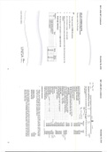
Investment and depreciation balance over time. That is, sf (k) = δk. This implies that ∆k = 0.
The level of k at which ∆k = 0 is called the steady state level of capital per worker and is denoted
by k ∗ . This process is illustrated in the figure below.
We now ask ourselves what happens to k ∗ if we change the saving rate s. Suppose we increase the
saving rate s, this results into an increase in sf (k). Therefore, the sf (k)-curve shifts upward. This
results into a new equilibrium sf (k) = δk at a higher steady state level of capital per worker k ∗ .
9
, 4.3 Golden rule level of capital
The steady state value of k that maximizes consumption is called the Golden Rule level of capital
∗
and is denoted by kgold . Recall that c = y − i = f (k) − sf (k). Since we only look for steady state
levels of capital per worker, we have that
∆k = 0 ⇔ sf (k) = δk
therefore the following holds for all steady state levels of capital per worker:
c∗ = y − i = f (k ∗ ) − sf (k ∗ ) = f (k ∗ ) − δk ∗
∗
Since we have to maximize consumption in order to find kgold we have to solve:
d
f (k ∗ ) − δk ∗ = 0
dk ∗
MPK − δ = 0
MPK = δ
Remember that in the [k, f (k)]-plane the slope of the graph of the f (k)-function equals the MPK.
∗
And the slope of the δk-line equals δ. We can find kgold by drawing the graph of f (k ∗ ) and the
∗
δk-line: the point at which the slope of the graph of f (k ) is equal to the slope of the δk-line is the
∗ ∗
Golden Rule level of capital kgold , since only then we have M P K = δ. We can then insert the kgold
into sf (k) = δk to find the saving rate s. This is also illustrated in the figure below.
√
Example: Let f (k) = k and let δ =
0.1. Find the saving rate s at the Golden
Rule level of capital.
Solution:
MPK = δ
∂f (k)
= 0.1
∂k
1
√ = 0.1
2 k
√
10 = 2 k
∗
kgold = 25
∗
We now insert kgold into sf (k) = δk
∗ ∗
sf (kgold ) = δkgold
√
s 25 = 0.1 ∗ 25
5s = 2.5
s = 0.5
∗ 1
The saving rate s at kgold is given by s = 2
10
Tim Eijkenaar
May 2020
1
,Contents
1 GDP Accounting 4
1.1 GDP . . . . . . . . . . . . . . . . . . . . . . . . . . . . . . . . . . . . . . . . . . . . . 4
1.2 Expenditure components of GDP . . . . . . . . . . . . . . . . . . . . . . . . . . . . . 4
1.3 Price indexes . . . . . . . . . . . . . . . . . . . . . . . . . . . . . . . . . . . . . . . . 4
2 Unemployment 5
2.1 Measuring joblessness . . . . . . . . . . . . . . . . . . . . . . . . . . . . . . . . . . . 5
2.2 The natural rate of unemployment . . . . . . . . . . . . . . . . . . . . . . . . . . . . 5
3 Economic growth 6
3.1 Production function . . . . . . . . . . . . . . . . . . . . . . . . . . . . . . . . . . . . 6
3.2 Cobb-Douglas production function . . . . . . . . . . . . . . . . . . . . . . . . . . . . 7
4 Solow growth model 8
4.1 The production function . . . . . . . . . . . . . . . . . . . . . . . . . . . . . . . . . . 8
4.2 Steady state level of capital . . . . . . . . . . . . . . . . . . . . . . . . . . . . . . . . 9
4.3 Golden rule level of capital . . . . . . . . . . . . . . . . . . . . . . . . . . . . . . . . 10
4.4 The effect of efficiency and population growth . . . . . . . . . . . . . . . . . . . . . . 12
5 Money and banking 13
5.1 Money . . . . . . . . . . . . . . . . . . . . . . . . . . . . . . . . . . . . . . . . . . . . 13
5.2 The quantity equation . . . . . . . . . . . . . . . . . . . . . . . . . . . . . . . . . . . 13
5.3 The demand for money . . . . . . . . . . . . . . . . . . . . . . . . . . . . . . . . . . 14
5.4 The Fisher effect . . . . . . . . . . . . . . . . . . . . . . . . . . . . . . . . . . . . . . 14
5.5 The cost of holding money . . . . . . . . . . . . . . . . . . . . . . . . . . . . . . . . . 15
5.6 Exchange rates . . . . . . . . . . . . . . . . . . . . . . . . . . . . . . . . . . . . . . . 15
6 Aggregate demand and supply 16
6.1 Aggregate demand . . . . . . . . . . . . . . . . . . . . . . . . . . . . . . . . . . . . . 16
6.2 Aggregate supply . . . . . . . . . . . . . . . . . . . . . . . . . . . . . . . . . . . . . . 17
6.3 Aggregate supply = aggregate demand . . . . . . . . . . . . . . . . . . . . . . . . . . 17
6.4 Shocks . . . . . . . . . . . . . . . . . . . . . . . . . . . . . . . . . . . . . . . . . . . . 18
7 IS-LM Model 19
7.1 IS-Curve . . . . . . . . . . . . . . . . . . . . . . . . . . . . . . . . . . . . . . . . . . 19
7.2 Shifting the IS-curve . . . . . . . . . . . . . . . . . . . . . . . . . . . . . . . . . . . . 20
7.3 LM -Curve . . . . . . . . . . . . . . . . . . . . . . . . . . . . . . . . . . . . . . . . . . 21
7.4 Shifting the LM -curve . . . . . . . . . . . . . . . . . . . . . . . . . . . . . . . . . . . 21
7.5 Equilibrium analysis . . . . . . . . . . . . . . . . . . . . . . . . . . . . . . . . . . . . 22
7.6 Multipliers . . . . . . . . . . . . . . . . . . . . . . . . . . . . . . . . . . . . . . . . . 23
8 Mundell-Fleming model 24
8.1 IS ∗ -curve . . . . . . . . . . . . . . . . . . . . . . . . . . . . . . . . . . . . . . . . . . 24
8.2 When do we shift the IS ∗ -curve? . . . . . . . . . . . . . . . . . . . . . . . . . . . . . 24
8.3 LM ∗ -curve . . . . . . . . . . . . . . . . . . . . . . . . . . . . . . . . . . . . . . . . . 25
2
, 8.4 When do we shift the LM ∗ curve? . . . . . . . . . . . . . . . . . . . . . . . . . . . . 25
8.5 Equilibrium analysis . . . . . . . . . . . . . . . . . . . . . . . . . . . . . . . . . . . . 26
8.6 Fixed exchange rates . . . . . . . . . . . . . . . . . . . . . . . . . . . . . . . . . . . . 27
8.7 Equilibrium analysis: e = e . . . . . . . . . . . . . . . . . . . . . . . . . . . . . . . . 27
9 Three models of aggregate supply 29
9.1 The sticky-price model . . . . . . . . . . . . . . . . . . . . . . . . . . . . . . . . . . . 29
9.2 The sticky-wage model . . . . . . . . . . . . . . . . . . . . . . . . . . . . . . . . . . . 30
9.3 Imperfect information model . . . . . . . . . . . . . . . . . . . . . . . . . . . . . . . 30
9.4 The new SRAS . . . . . . . . . . . . . . . . . . . . . . . . . . . . . . . . . . . . . . . 30
10 Phillips curve 31
3
,1 GDP Accounting
1.1 GDP
Let Qi,t denote the quantity of product i at year t and let Pi,t be the price of product i at year t.
Assume the chosen base year is t = 0. Then,
X
Real GDP at year t = Pi,0 ∗ Qi,t
i
X
Nominal GDP at year t = Pi,t ∗ Qi,t
i
1.2 Expenditure components of GDP
The four expenditure components of GDP are given by the following formula: Y = C + I + G + N X
Y = Output = Income = GDP
C = Consumption = C(Y − T )
I = Investment = I(r)
G = Government spending
N X = Net exports = N X(e)
Where we used the fact that output Y is a function of disposable income (Y − T ), investment I is
a function of the interest rate r and N X is a function of the exchange rate e.
We define:
Trade deficit = X − M = Exports − Imports
Capital inflow = −N X
Furthermore we have the following formulas where we assume a closed economy (N X = 0):
Private saving = Y − T − C
Public saving = T − G
Saving = S = (Y − T − C) + (T − G) = I
1.3 Price indexes
Both the Paasche price index and the Laspeyres price index reflect what is happening to the price
level in the economy. They are defined in the following way.
P
Nominal GDP at year t Pi,t ∗ Qi,t
Paasche price index = GDP Deflator = = Pi
Real GDP at year t i Pi,0 ∗ Qi,t
P
P i,t ∗ Qi,0
Laspeyres price index = CPI = P i
i P i,0 ∗ Q i,0
4
,2 Unemployment
2.1 Measuring joblessness
Each adult is placed into one of the following three categories:
1. Employed E
2. Unemployed U
3. Not in the labour force
We define
Labour force = Number of employed + Number of unemployed
Number of employed
Unemployment rate = ∗ 100%
Labour force
Labour force
Labour force participation rate = ∗ 100%
Adult population
2.2 The natural rate of unemployment
It is reasonable to assume that the labour force L is fixed. The unemployment rate is under this
assumption fully determined by the transition of individuals in the labour force. Let s denote the
rate of job separation and let f denote the rate of job finding. Then the number of people that lose
their job sE must be equal to the number of people that find a new job f U .
f U = sE
f U = s(L − U )
U 1
=
L 1 + f/s
Where we used the fact that E = L − U and did some basic algebra steps to derive the last formula.
5
,3 Economic growth
3.1 Production function
Output Y , or GDP, is a function of the amount of capital K and the amount of labour L.
That is, Y = F (K, L).
A production function has the property ’constant returns to scale’ if zY = F (zK, zL) for every real
number z.
The marginal product of labour M P L is the extra amount of output a firm gets given a unit change
in the amount of labour. That is, M P L is the partial derivative of F with respect to L:
∂F (K, L)
MPL =
∂L
Likewise, the marginal product of capital M P K is the change in the amount of output given a unit
change in the amount of capital:
∂F (K, L)
MPK =
∂K
The above gives us the following result: let P be the price of one single unit of output and let W
be the wage corresponding to one unit of labour. Then if we increase L by one unit:
∆Profit = ∆Revenues − ∆Cost
= MPL ∗ P − W
Intuitively, as long as ∆Profit > 0 we want to increase the amount of labour until ∆Profit = 0.
Therefore, every competitive firm will satisfy
∆Profit = ∆Revenues − ∆Cost
0 = MPL ∗ P − W
W
MPL =
P
We can do the same steps for the M P K. This will lead us to the following result:
R
MPK =
P
6
,3.2 Cobb-Douglas production function
Any production function of the form F (K, L) = A K α L1−α with A > 0 and 0 ≤ α ≤ 1 is called a
’Cobb-Douglas production function’.
Note that F has constant return to scale since
F (zK, zL) = A(zK)α (zL)1−α = AK α L1−α z α z 1−α = zA K α L1−α = zF (K, L)
Furthermore for every Cobb-Douglas production function it holds that
Y
M P L = (1 − α)AK α L−α = (1 − α)
L
Y
M P K = αAK α−1 L1−α = α
K
7
,4 Solow growth model
4.1 The production function
Recall that the production function is given by F (K, L). In the Solow growth model we assume
that F has constant return to scale: zF (K, L) = F (zK, zL). Furthermore, we want to analyse
all quantities in the economy relative to the size of the labour force. That means that we are not
interested in output Y itself, but in YL . We now rewrite Y = F (K, L) to know more about YL . We
use the fact that F has constant return to scale. Note that in this case z = L1 :
Y = F (K, L)
Y F (K, L)
=
L L
K L
= F( , )
L L
K
= F( , 1)
L
From now on, we denote every variable relative to the size of the labour force with just the small
letter of the variable:
Y K C
=y =k =c
L L L
We can now rewrite our production function. Note that we can simply forget about the variable ’1’
since it is a constant. We use f instead of F for convenience.
Y K
= F ( , 1)
L L
y = F (k, 1)
= f (k)
8
,4.2 Steady state level of capital
In the Solow growth model output per worker y is divided between consumption per worker c
and investment per worker i. We assume a closed economy (N X = 0) and we ignore government
spending G:
y =c+i
We assume that individuals save a fraction s of their income (s ∈ [0, 1]) and consume a fraction
(1 − s) of their income:
c = (1 − s)y = (1 − s)f (k) i = sy = sf (k)
The capital stock changes over time because of the impact investment i and depreciation δ have on
it. Let i be the investment per worker per year and let δ be the fraction of capital that depreciates
per year. Then
∆k = i − δk = sf (k) − δk
Investment and depreciation balance over time. That is, sf (k) = δk. This implies that ∆k = 0.
The level of k at which ∆k = 0 is called the steady state level of capital per worker and is denoted
by k ∗ . This process is illustrated in the figure below.
We now ask ourselves what happens to k ∗ if we change the saving rate s. Suppose we increase the
saving rate s, this results into an increase in sf (k). Therefore, the sf (k)-curve shifts upward. This
results into a new equilibrium sf (k) = δk at a higher steady state level of capital per worker k ∗ .
9
, 4.3 Golden rule level of capital
The steady state value of k that maximizes consumption is called the Golden Rule level of capital
∗
and is denoted by kgold . Recall that c = y − i = f (k) − sf (k). Since we only look for steady state
levels of capital per worker, we have that
∆k = 0 ⇔ sf (k) = δk
therefore the following holds for all steady state levels of capital per worker:
c∗ = y − i = f (k ∗ ) − sf (k ∗ ) = f (k ∗ ) − δk ∗
∗
Since we have to maximize consumption in order to find kgold we have to solve:
d
f (k ∗ ) − δk ∗ = 0
dk ∗
MPK − δ = 0
MPK = δ
Remember that in the [k, f (k)]-plane the slope of the graph of the f (k)-function equals the MPK.
∗
And the slope of the δk-line equals δ. We can find kgold by drawing the graph of f (k ∗ ) and the
∗
δk-line: the point at which the slope of the graph of f (k ) is equal to the slope of the δk-line is the
∗ ∗
Golden Rule level of capital kgold , since only then we have M P K = δ. We can then insert the kgold
into sf (k) = δk to find the saving rate s. This is also illustrated in the figure below.
√
Example: Let f (k) = k and let δ =
0.1. Find the saving rate s at the Golden
Rule level of capital.
Solution:
MPK = δ
∂f (k)
= 0.1
∂k
1
√ = 0.1
2 k
√
10 = 2 k
∗
kgold = 25
∗
We now insert kgold into sf (k) = δk
∗ ∗
sf (kgold ) = δkgold
√
s 25 = 0.1 ∗ 25
5s = 2.5
s = 0.5
∗ 1
The saving rate s at kgold is given by s = 2
10