NORMAL DISTRIBUTION DETAIL TUTORIAL
Normal Distribution
The normal distribution is a distribution that can be described by the mean and the
standard deviation in a symmetric manner. It is often referred to as a 'bell curve'
because of its shape:
CHARACTERISTICS OF THE NORMAL DISTRIBUTION
• Most of the data or values are around the mean(center)
• The median and mean are equal (central tendency theorem)
• It has only one mode
• It is symmetric, that’s the same amount of decrease on the left and the right of
the center
• The area under the curve of the normal distribution represents probabilities for
the data.
NB
Many observed frequency distributions do approximate the normal curve. The normal
curve can be used to obtain answers to a wide variety of questions.
There are infinite numbers of normal curves, each with its own mean and standard
deviation but a standard normal curve always has a mean of 0 and a standard deviation
of 1.
We can always convert a normal curve to the standard normal curve or distribution.
Types of normal curve problems:
(1) those that require you to find the unknown proportion (of area) associated with some
score or pair of scores. Which normally require you to convert original scores
X−μ
into z scores = σ
(2) those that require you to find the unknown score or scores associated with some
area. Which usually require you to translate a z score back into an original score
X=μ+Zσ
, Tests Involving the Normal Distribution
• One-Tailed and Two-Tailed Tests
At a particular confidence interval, and depending whether a one tail or two tail test, the
z results should be within a range read from tables. A value outside the range can lead
to a rejection of the hypothesis that at the chosen confident interval, the data is not a
normal curve.
A 90% (0.95) confidence interval is the same as a 0.05 level of significance
HYPOTHESIS: Assuming sampling distribution of a statistic S is a normal distribution
with mean and standard deviation. we can be 95% confident that, if the hypothesis is
true, the z score of an actual sample statistic S will lie between -1.96 and 1.96 (since
the area under the normal curve between these values is 0.95)
• Reject the hypothesis at a 0.05 level of significance if the z score of the statistic S
lies outside the range 1.96 to 1.96 (i.e., either z =1.96 or z =1.96). This is
equivalent to saying that the observed sample statistic is significant at the 0.05
level.
• Accept the hypothesis (or, if desired, make no decision at all) otherwise
(i) The parameter is greater than the stated value (right-tailed test).
(ii) The parameter is less than the stated value (left-tailed test).
(iii) The parameter is either greater than or less than the stated value (two-tailed test)
Normal Distribution
The normal distribution is a distribution that can be described by the mean and the
standard deviation in a symmetric manner. It is often referred to as a 'bell curve'
because of its shape:
CHARACTERISTICS OF THE NORMAL DISTRIBUTION
• Most of the data or values are around the mean(center)
• The median and mean are equal (central tendency theorem)
• It has only one mode
• It is symmetric, that’s the same amount of decrease on the left and the right of
the center
• The area under the curve of the normal distribution represents probabilities for
the data.
NB
Many observed frequency distributions do approximate the normal curve. The normal
curve can be used to obtain answers to a wide variety of questions.
There are infinite numbers of normal curves, each with its own mean and standard
deviation but a standard normal curve always has a mean of 0 and a standard deviation
of 1.
We can always convert a normal curve to the standard normal curve or distribution.
Types of normal curve problems:
(1) those that require you to find the unknown proportion (of area) associated with some
score or pair of scores. Which normally require you to convert original scores
X−μ
into z scores = σ
(2) those that require you to find the unknown score or scores associated with some
area. Which usually require you to translate a z score back into an original score
X=μ+Zσ
, Tests Involving the Normal Distribution
• One-Tailed and Two-Tailed Tests
At a particular confidence interval, and depending whether a one tail or two tail test, the
z results should be within a range read from tables. A value outside the range can lead
to a rejection of the hypothesis that at the chosen confident interval, the data is not a
normal curve.
A 90% (0.95) confidence interval is the same as a 0.05 level of significance
HYPOTHESIS: Assuming sampling distribution of a statistic S is a normal distribution
with mean and standard deviation. we can be 95% confident that, if the hypothesis is
true, the z score of an actual sample statistic S will lie between -1.96 and 1.96 (since
the area under the normal curve between these values is 0.95)
• Reject the hypothesis at a 0.05 level of significance if the z score of the statistic S
lies outside the range 1.96 to 1.96 (i.e., either z =1.96 or z =1.96). This is
equivalent to saying that the observed sample statistic is significant at the 0.05
level.
• Accept the hypothesis (or, if desired, make no decision at all) otherwise
(i) The parameter is greater than the stated value (right-tailed test).
(ii) The parameter is less than the stated value (left-tailed test).
(iii) The parameter is either greater than or less than the stated value (two-tailed test)