CASE - Econometrie - 2024/2025
INFERENTIE
[INPUT]
myseed <- 252
set.seed(myseed)
# Document inlezen en random size van 250 selecteren
house_data <- read.csv("Huisprijzen.csv", header = TRUE, dec = ",", sep = ";")
selectedobs <- sample.int(nrow(house_data), size = 250, replace = FALSE)
sampled_house_data <- house_data[selectedobs,]
View(sampled_house_data)
[INPUT]
# Scheve verdeling, dus transformatie uitvoeren. Log_prijs heeft normaal verdeelde
# histogram en kleinere getallen
hist(sampled_house_data$price, main = "Histogram van huisprijs", xlab =
"Huisprijs")
sampled_house_data$log_price <- log(sampled_house_data$price)
hist(sampled_house_data$log_price, main = "Gecorrigeerde histogram met log_prijs"
, xlab = "Log_prijs")
[OUTPUT]
[INPUT]
numeric_data <- sampled_house_data[sapply(sampled_house_data, is.numeric)]
print(numeric_data)
cor_matrix <- cor(numeric_data, use = "complete.obs")
print(cor_matrix)
[OUTPUT]
Luca Pleysier - Econometrie Case - 24/25
, [INPUT]
str(sampled_house_data)
categorical_vars <- names(sampled_house_data)[sapply(sampled_house_data,
function(x)is.character(x) || is.factor(x))]
print(categorical_vars)
[OUTPUT]
[INPUT]
# Categorische variabelen omzetten in dummies, aangezien lineair regressiemodel
# niet direct kan omgaan met deze variabelen. -1 omdat R anders automatisch een
# referentiecategorie opneemt tegen multicollineariteit.
lapply(sampled_house_data[categorical_vars], unique)
dummy_matrix <- model.matrix(~heating + fuel + sewer + waterfront +
newConstruction + centralAir - 1, data =
sampled_house_data)
head(dummy_matrix)
[OUTPUT]
[INPUT]
# Correlaties tussen log_price en categorische en numerieke variabelen
combined_data <- cbind(log_price = sampled_house_data$log_price
, sampled_house_data[,c("lotSize", "age", "landValue",
"livingArea", "pctCollege", "bedrooms", "fireplaces",
"bathrooms", "rooms")], dummy_matrix)
cor_matrix_full <- cor(combined_data, use = "complete.obs")
log_price_cor <- cor_matrix_full[1,]
log_price_cor_matrix <- cor_matrix_full["log_price",,drop = FALSE]
log_price_cor <- cor_matrix_full["log_price",]
library(ggplot2)
cor_data <- data.frame(Variable = names(log_price_cor), Correlation =
log_price_cor)
ggplot(cor_data, aes(x = reorder(Variable, Correlation), y = Correlation)) +
geom_bar(stat = "identity", fill = "blue") + coord_flip() + labs(title =
"Correlaties met log_price", x = "Variabelen", y = "Correlatie") +
theme_minimal()
Luca Pleysier - Econometrie Case - 24/25
INFERENTIE
[INPUT]
myseed <- 252
set.seed(myseed)
# Document inlezen en random size van 250 selecteren
house_data <- read.csv("Huisprijzen.csv", header = TRUE, dec = ",", sep = ";")
selectedobs <- sample.int(nrow(house_data), size = 250, replace = FALSE)
sampled_house_data <- house_data[selectedobs,]
View(sampled_house_data)
[INPUT]
# Scheve verdeling, dus transformatie uitvoeren. Log_prijs heeft normaal verdeelde
# histogram en kleinere getallen
hist(sampled_house_data$price, main = "Histogram van huisprijs", xlab =
"Huisprijs")
sampled_house_data$log_price <- log(sampled_house_data$price)
hist(sampled_house_data$log_price, main = "Gecorrigeerde histogram met log_prijs"
, xlab = "Log_prijs")
[OUTPUT]
[INPUT]
numeric_data <- sampled_house_data[sapply(sampled_house_data, is.numeric)]
print(numeric_data)
cor_matrix <- cor(numeric_data, use = "complete.obs")
print(cor_matrix)
[OUTPUT]
Luca Pleysier - Econometrie Case - 24/25
, [INPUT]
str(sampled_house_data)
categorical_vars <- names(sampled_house_data)[sapply(sampled_house_data,
function(x)is.character(x) || is.factor(x))]
print(categorical_vars)
[OUTPUT]
[INPUT]
# Categorische variabelen omzetten in dummies, aangezien lineair regressiemodel
# niet direct kan omgaan met deze variabelen. -1 omdat R anders automatisch een
# referentiecategorie opneemt tegen multicollineariteit.
lapply(sampled_house_data[categorical_vars], unique)
dummy_matrix <- model.matrix(~heating + fuel + sewer + waterfront +
newConstruction + centralAir - 1, data =
sampled_house_data)
head(dummy_matrix)
[OUTPUT]
[INPUT]
# Correlaties tussen log_price en categorische en numerieke variabelen
combined_data <- cbind(log_price = sampled_house_data$log_price
, sampled_house_data[,c("lotSize", "age", "landValue",
"livingArea", "pctCollege", "bedrooms", "fireplaces",
"bathrooms", "rooms")], dummy_matrix)
cor_matrix_full <- cor(combined_data, use = "complete.obs")
log_price_cor <- cor_matrix_full[1,]
log_price_cor_matrix <- cor_matrix_full["log_price",,drop = FALSE]
log_price_cor <- cor_matrix_full["log_price",]
library(ggplot2)
cor_data <- data.frame(Variable = names(log_price_cor), Correlation =
log_price_cor)
ggplot(cor_data, aes(x = reorder(Variable, Correlation), y = Correlation)) +
geom_bar(stat = "identity", fill = "blue") + coord_flip() + labs(title =
"Correlaties met log_price", x = "Variabelen", y = "Correlatie") +
theme_minimal()
Luca Pleysier - Econometrie Case - 24/25