Samenvatting Econometrics
Economists are often interested in (causal) relations between variables or comparisons between
different populations. The relationship can be between individuals or over time. A causal effect is
the direct effect of x on y. There are three types of statistical methods to draw statistical
inferences about the characteristics of the full population: 1) estimation 2) hypothesis testing and
3) confidence intervals. U is the disturbance/error term: the difference between y and the
population regression line. U is different for everyone because the equation describes the
regression line with identical betas for everyone.
DISTRIBUTION
Location: expected value (mean) of a random variable. Y: E[Y]=𝜇"
Spread: variance of Y: var(Y)=E[(Y-𝜇" )2]=𝜎 $ " . Measures the dispersion of the distribution.
Standard deviation of Y: 𝜎"
%[(()*+ )-]
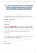
Shape: skewness of the distribution of Y = /- +
. It tells how much the distribution disperse
from a normal distribution (skewness = 0). Otherwise there is a lack of symmetry.
%[(()*+ )0 ]
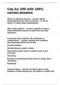
Tail: kurtosis of the distribution of Y: /0 +
. A lot of mass in the tails (normal = 3) tells that the
variance is made up by some extreme values/outliers (high = 7).
The covariance gives the relationship between two random variables:
𝑐𝑜𝑣(𝑋, 𝑌) = 𝜎8" = 𝐸[(𝑋 − 𝐸[𝑋])(𝑌 − 𝐸[𝑌])]
The correlation is a standardized version of the covariance:
?@A(8,")
−1 ≤ 𝑐𝑜𝑟𝑟(𝑋, 𝑌) = 𝜌8" = / / ≤ 1
B +
Simple random sampling: n objects are drawn at random from a population and each object is
equally likely to be drawn:
- The n observations in the sample are denoted Y1,…,Yn
- Under simple random sampling, Y1 is distributed independently of Y2,…,Yn
- Because Y1,…,Yn are randomly drawn from the same population, the marginal distribution
of Yi is the same for each i =1,…,n, i.e. Y1,…,Yn are identically distributed
- When Y1,…,Yn are independently distributed and drawn from the same distributed, they
are independently and identically distributed (i.i.d.)
Asymptotic distribution: approximation to the sampling distribution that relies on the sample size
being large. Two key tools are used:
1. Law of large numbers: when n is large, the sample average will be close to the actual
mean with very high probability. It converges. The sample is consistent with the actual.
2. Central limit theory: when n is large, the distribution of the sample average is well
approximated by a normal distribution, i.e. the sample average has an asymptotic normal
distribution, and the distribution of the standardized version of the sample average is well
approximated by a standard normal distribution.
Key insight of statistics: one can learn about the population distribution by selecting a random
sample from that population. Using statistical methods, the random sample can be used to draw
statistical inferences about characteristics of the full populations. There are three types:
1. Estimation: entails computing a best guess numerical value for an unknown characteristic
of a population distribution from a sample of data
, 2. Hypothesis testing: entails formulating a specific hypothesis about the population, then
using sample evidence to decide whether it is true
3. Confidence intervals: use a sample of data to estimate an interval for an unknown
population characteristic
An estimator is a function of a sample of data to be drawn randomly from a population used to
infer an estimate for an unknown parameter. An estimator is a random variable because of the
randomness in selecting the sample, while an estimate is a nonrandom number. An estimate is
the numerical value of the estimator when it is actually computed using data from a specific
sample.
The desirable properties:
- Unbiasedness: the mean of the sampling distribution is equal to the estimation; sample
mean = population mean. Small sample property. The estimator has lack of bias, is thus
unbiased. It holds for any sample size. The expected value (mean of sample distribution) is
equal to the true unknown population.
- Consistency: as the sample size increases, the sampling distribution of the estimator
becomes increasingly concentrated at the true parameter value. The estimator is
consistent and holds if the sample is large (asymptotic property). When the sample size
increases, it comes closer to the population size and the estimator converges in the
probability into a true characteristic.
- Efficiency: the estimator has the smallest variance among the unbiased estimators. The
lower the variance, the more efficient and more precise the variable is. Most precise in
small samples.
The Best Linear Unbiased Estimator (BLUE) is the best variable to use, it meets all three
properties.
Hypothesis testing. The null hypothesis is that the population mean takes on a specific value. The
two-sided alternative hypothesis specifies what is true if the null hypothesis is not. Type I error is
when the null hypothesis is rejected when in fact it is true. Type II error is when the null
hypothesis is not rejected when in fact it is not true. The t-statistic is a statistic used to perform a
hypothesis test.
An endogenous regressor is one that is correlated with the error term. An exogenous regressor is
uncorrelated with the error term. Reasons why a regressor can be endogenous are: reversed
causality, omitted variables, errors-in-variables.
Interpreting:
Economists are often interested in (causal) relations between variables or comparisons between
different populations. The relationship can be between individuals or over time. A causal effect is
the direct effect of x on y. There are three types of statistical methods to draw statistical
inferences about the characteristics of the full population: 1) estimation 2) hypothesis testing and
3) confidence intervals. U is the disturbance/error term: the difference between y and the
population regression line. U is different for everyone because the equation describes the
regression line with identical betas for everyone.
DISTRIBUTION
Location: expected value (mean) of a random variable. Y: E[Y]=𝜇"
Spread: variance of Y: var(Y)=E[(Y-𝜇" )2]=𝜎 $ " . Measures the dispersion of the distribution.
Standard deviation of Y: 𝜎"
%[(()*+ )-]
Shape: skewness of the distribution of Y = /- +
. It tells how much the distribution disperse
from a normal distribution (skewness = 0). Otherwise there is a lack of symmetry.
%[(()*+ )0 ]
Tail: kurtosis of the distribution of Y: /0 +
. A lot of mass in the tails (normal = 3) tells that the
variance is made up by some extreme values/outliers (high = 7).
The covariance gives the relationship between two random variables:
𝑐𝑜𝑣(𝑋, 𝑌) = 𝜎8" = 𝐸[(𝑋 − 𝐸[𝑋])(𝑌 − 𝐸[𝑌])]
The correlation is a standardized version of the covariance:
?@A(8,")
−1 ≤ 𝑐𝑜𝑟𝑟(𝑋, 𝑌) = 𝜌8" = / / ≤ 1
B +
Simple random sampling: n objects are drawn at random from a population and each object is
equally likely to be drawn:
- The n observations in the sample are denoted Y1,…,Yn
- Under simple random sampling, Y1 is distributed independently of Y2,…,Yn
- Because Y1,…,Yn are randomly drawn from the same population, the marginal distribution
of Yi is the same for each i =1,…,n, i.e. Y1,…,Yn are identically distributed
- When Y1,…,Yn are independently distributed and drawn from the same distributed, they
are independently and identically distributed (i.i.d.)
Asymptotic distribution: approximation to the sampling distribution that relies on the sample size
being large. Two key tools are used:
1. Law of large numbers: when n is large, the sample average will be close to the actual
mean with very high probability. It converges. The sample is consistent with the actual.
2. Central limit theory: when n is large, the distribution of the sample average is well
approximated by a normal distribution, i.e. the sample average has an asymptotic normal
distribution, and the distribution of the standardized version of the sample average is well
approximated by a standard normal distribution.
Key insight of statistics: one can learn about the population distribution by selecting a random
sample from that population. Using statistical methods, the random sample can be used to draw
statistical inferences about characteristics of the full populations. There are three types:
1. Estimation: entails computing a best guess numerical value for an unknown characteristic
of a population distribution from a sample of data
, 2. Hypothesis testing: entails formulating a specific hypothesis about the population, then
using sample evidence to decide whether it is true
3. Confidence intervals: use a sample of data to estimate an interval for an unknown
population characteristic
An estimator is a function of a sample of data to be drawn randomly from a population used to
infer an estimate for an unknown parameter. An estimator is a random variable because of the
randomness in selecting the sample, while an estimate is a nonrandom number. An estimate is
the numerical value of the estimator when it is actually computed using data from a specific
sample.
The desirable properties:
- Unbiasedness: the mean of the sampling distribution is equal to the estimation; sample
mean = population mean. Small sample property. The estimator has lack of bias, is thus
unbiased. It holds for any sample size. The expected value (mean of sample distribution) is
equal to the true unknown population.
- Consistency: as the sample size increases, the sampling distribution of the estimator
becomes increasingly concentrated at the true parameter value. The estimator is
consistent and holds if the sample is large (asymptotic property). When the sample size
increases, it comes closer to the population size and the estimator converges in the
probability into a true characteristic.
- Efficiency: the estimator has the smallest variance among the unbiased estimators. The
lower the variance, the more efficient and more precise the variable is. Most precise in
small samples.
The Best Linear Unbiased Estimator (BLUE) is the best variable to use, it meets all three
properties.
Hypothesis testing. The null hypothesis is that the population mean takes on a specific value. The
two-sided alternative hypothesis specifies what is true if the null hypothesis is not. Type I error is
when the null hypothesis is rejected when in fact it is true. Type II error is when the null
hypothesis is not rejected when in fact it is not true. The t-statistic is a statistic used to perform a
hypothesis test.
An endogenous regressor is one that is correlated with the error term. An exogenous regressor is
uncorrelated with the error term. Reasons why a regressor can be endogenous are: reversed
causality, omitted variables, errors-in-variables.
Interpreting: