Week 1: Frequency Data, Chi-Squared & Trigonometry | Writing Methods/Results 1
Pearson’s Chi-squared test:
1. First need to come up with our expected counts under the null hypothesis [e.g if the null is that
they’re all the same, then this is just the total count split across the categories]
2. Take the difference between each count & its expected under the null hypothesis, square them
deviation = sum(observed - model or expected)^2], divide by the expected
3. add them up to obtain the chi-squared statistic
4. Df = (no of rows - 1) * (no of columns -1)
Model = expected frequencies - calculated for each of the cells in the contingency table:
○ Model = row total x column total / n (no of total observations)
● Used to see if there’s a relationship between two categorical variables [e.g if you failed or
passed, if you are dead or alive = you can be in only one category]
Assumptions:
➔ Independence = each person/item contributes to only one cell of the contingency table
➔ expected frequencies should be greater than 5. In larger contingency tables no expected
frequencies should be below 1. If it does then use Fisher’s exact test.
➔ If N increases then there’s a greater chance of seeing a significant effect
Degrees of freedom and chi-squared distribution
● The mean of a categorical variable is meaningless - so
always analyse frequencies
● The chi-squared distribution is a probability distribution. It’s
denoted as x^2
● x^2(i) -> x^2 is the chi-squared value and i is the df
● Df determines the shape, location & spread of distribution
● The chi-squared statistic is distributed according to a
specific distribution under the null hypothesis, which is known as
the chi-squared distribution. The shape of the distribution
depends on the number of degrees of freedom
● Chi-squared is positively skewed [curves to the left - starts
big then decreases] & takes only non-negative values. As df
increases, shape of distribution becomes more symmetric -> normal distribution
Contingency tables & the two-way test
➔ Another use of chi-squared - to ask whether 2 categorical variables are related to one another
➔ Relationship between 2 categorical variables
➔ The standard way to represent data from a categorical analysis is through a contingency tables -
contingency tables uses proportions instead of raw nos - easy to compare visually
➔ Chi-squared -> test whether observed frequencies are different from expected frequencies
,Standardised residuals
➢ When we find a significant effect with the chi-squared test, this tells us that the data is unlikely
under the null hypothesis, but doesn’t tell us how the data differs
➢ How the data differ from wat we would expect under the null hypothesis = examine the residuals
from the model which reflects the deviation of the data [observed frequencies] from the model
[expected frequencies] in each cell = look at standardised residuals instead
➢ Standardised residuals can be interpreted as Z-scores
➢ standardized residuals are a measure of the difference between observed and expected
frequencies in each cell of a contingency table.
➢ Large standardized residuals indicate that the observed frequency is significantly different from
the expected frequency, suggesting a significant association between the variables being
studied.
Odds ratio: relative likelihood of different outcomes in the contingency table = Effect size
Test statistic
● Checked against a distribution with Degrees of freedom = (row - 1) x (column - 1)
● If it’s significant then there’s a significant association between the categorical variables in the
population
● The test distribution is approximate so in small samples use Fisher’s exact test
Likelihood Ratio Statistic
● An alternative to Pearson’s chi-squared, based on maximum-likelihood theory
● Create a model for which the probability of obtaining the observed set of data is maximised
● This model is compared to the probability of those data under the null hypothesis [model?]
● The resulting statistic compared observed frequencies with those predicted by the model
● i = rows. j = columns of the contingency table
● In is the natural logarithm
● Test statistics:
○ Has a chi-squared distribution with (r-1)*(c-1) degrees of freedom
○ Preferred to chi-square when samples are small
● Df determines the shape of the statistic curve
○ Low df [2x2 contingency table] = 1df = peak of curve moves more to right
● More df = high chi-squared value
● Residuals = difference between model and observed value
● Effect size for chi-square = odds ratio
, Reporting chi-squared: There was a significant association between type of training & whether or not
cats would dance x^2(1 [df]) = 25, p<.001. This represents the fact that, based on the odds ratio, the
odds of cats dancing were 6(2,16) times higher if they were trained with food than if trained with
affection
Code:
● packages : library() -> Tidyverse, gmodels, MASS
● Contingency table:
CrossTable(contingencyTable, fisher = TRUE, chisq = true, expected =TRUE, sresid = TRUE, format =
“SAS”/”SPSS”)
Maths from week 1:
● Sine = Opp/Hyp SOH
● Cosine = ADJ/HYP CAH
● Tangent [tan] = Opp/Adj = sine/cos TOA
Pythagoras’ theorem:
c^2 = b^2 + a^2
Opp^2 + Adj^2 = Hyp^2
Degrees & radians conversion:
❖ 1 rad = 360/2𝛑
❖ 1° = 2𝛑/360
❖ 1 radian = 180°/𝛑
How do the functions relate to each other?
★ sin(x) = cos(x-𝛑/2)
★ sin(-x) = -sin(x)
★ cos(-x) = cos(x)
★ tan(x) = sin(x)/cos(x)
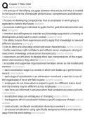
Week 2:
● GLM - general linear model - GLM predicts what is measured [DV = y-axis] from what’s
manipulated [IV - x-axis] -> normal graph with IV and DV showing a linear relationship [straight
line = positive or negative = strong relationship]
● Outcome = model + error [model that predicts your data and also other data sets -
generalisation]
LINEAR REGRESSION
➔ Can use GLMl to describe the relation between two variables & decide whether the relationship
is statistically significant
➔ GLM also allows to predict the value of the dependent variable given some new value(s) of the
independent variable(s).
➔ GLM allows to build models that incorporate multiple independent variables, whereas the
correlation coefficient can only describe the relationship between two individual variables.
➔ The specific version of the GLM that we use for this is referred to as linear regression.
➔ The simplest version of the linear regression model (with a single independent variable) can be
expressed as follows:
Pearson’s Chi-squared test:
1. First need to come up with our expected counts under the null hypothesis [e.g if the null is that
they’re all the same, then this is just the total count split across the categories]
2. Take the difference between each count & its expected under the null hypothesis, square them
deviation = sum(observed - model or expected)^2], divide by the expected
3. add them up to obtain the chi-squared statistic
4. Df = (no of rows - 1) * (no of columns -1)
Model = expected frequencies - calculated for each of the cells in the contingency table:
○ Model = row total x column total / n (no of total observations)
● Used to see if there’s a relationship between two categorical variables [e.g if you failed or
passed, if you are dead or alive = you can be in only one category]
Assumptions:
➔ Independence = each person/item contributes to only one cell of the contingency table
➔ expected frequencies should be greater than 5. In larger contingency tables no expected
frequencies should be below 1. If it does then use Fisher’s exact test.
➔ If N increases then there’s a greater chance of seeing a significant effect
Degrees of freedom and chi-squared distribution
● The mean of a categorical variable is meaningless - so
always analyse frequencies
● The chi-squared distribution is a probability distribution. It’s
denoted as x^2
● x^2(i) -> x^2 is the chi-squared value and i is the df
● Df determines the shape, location & spread of distribution
● The chi-squared statistic is distributed according to a
specific distribution under the null hypothesis, which is known as
the chi-squared distribution. The shape of the distribution
depends on the number of degrees of freedom
● Chi-squared is positively skewed [curves to the left - starts
big then decreases] & takes only non-negative values. As df
increases, shape of distribution becomes more symmetric -> normal distribution
Contingency tables & the two-way test
➔ Another use of chi-squared - to ask whether 2 categorical variables are related to one another
➔ Relationship between 2 categorical variables
➔ The standard way to represent data from a categorical analysis is through a contingency tables -
contingency tables uses proportions instead of raw nos - easy to compare visually
➔ Chi-squared -> test whether observed frequencies are different from expected frequencies
,Standardised residuals
➢ When we find a significant effect with the chi-squared test, this tells us that the data is unlikely
under the null hypothesis, but doesn’t tell us how the data differs
➢ How the data differ from wat we would expect under the null hypothesis = examine the residuals
from the model which reflects the deviation of the data [observed frequencies] from the model
[expected frequencies] in each cell = look at standardised residuals instead
➢ Standardised residuals can be interpreted as Z-scores
➢ standardized residuals are a measure of the difference between observed and expected
frequencies in each cell of a contingency table.
➢ Large standardized residuals indicate that the observed frequency is significantly different from
the expected frequency, suggesting a significant association between the variables being
studied.
Odds ratio: relative likelihood of different outcomes in the contingency table = Effect size
Test statistic
● Checked against a distribution with Degrees of freedom = (row - 1) x (column - 1)
● If it’s significant then there’s a significant association between the categorical variables in the
population
● The test distribution is approximate so in small samples use Fisher’s exact test
Likelihood Ratio Statistic
● An alternative to Pearson’s chi-squared, based on maximum-likelihood theory
● Create a model for which the probability of obtaining the observed set of data is maximised
● This model is compared to the probability of those data under the null hypothesis [model?]
● The resulting statistic compared observed frequencies with those predicted by the model
● i = rows. j = columns of the contingency table
● In is the natural logarithm
● Test statistics:
○ Has a chi-squared distribution with (r-1)*(c-1) degrees of freedom
○ Preferred to chi-square when samples are small
● Df determines the shape of the statistic curve
○ Low df [2x2 contingency table] = 1df = peak of curve moves more to right
● More df = high chi-squared value
● Residuals = difference between model and observed value
● Effect size for chi-square = odds ratio
, Reporting chi-squared: There was a significant association between type of training & whether or not
cats would dance x^2(1 [df]) = 25, p<.001. This represents the fact that, based on the odds ratio, the
odds of cats dancing were 6(2,16) times higher if they were trained with food than if trained with
affection
Code:
● packages : library() -> Tidyverse, gmodels, MASS
● Contingency table:
CrossTable(contingencyTable, fisher = TRUE, chisq = true, expected =TRUE, sresid = TRUE, format =
“SAS”/”SPSS”)
Maths from week 1:
● Sine = Opp/Hyp SOH
● Cosine = ADJ/HYP CAH
● Tangent [tan] = Opp/Adj = sine/cos TOA
Pythagoras’ theorem:
c^2 = b^2 + a^2
Opp^2 + Adj^2 = Hyp^2
Degrees & radians conversion:
❖ 1 rad = 360/2𝛑
❖ 1° = 2𝛑/360
❖ 1 radian = 180°/𝛑
How do the functions relate to each other?
★ sin(x) = cos(x-𝛑/2)
★ sin(-x) = -sin(x)
★ cos(-x) = cos(x)
★ tan(x) = sin(x)/cos(x)
Week 2:
● GLM - general linear model - GLM predicts what is measured [DV = y-axis] from what’s
manipulated [IV - x-axis] -> normal graph with IV and DV showing a linear relationship [straight
line = positive or negative = strong relationship]
● Outcome = model + error [model that predicts your data and also other data sets -
generalisation]
LINEAR REGRESSION
➔ Can use GLMl to describe the relation between two variables & decide whether the relationship
is statistically significant
➔ GLM also allows to predict the value of the dependent variable given some new value(s) of the
independent variable(s).
➔ GLM allows to build models that incorporate multiple independent variables, whereas the
correlation coefficient can only describe the relationship between two individual variables.
➔ The specific version of the GLM that we use for this is referred to as linear regression.
➔ The simplest version of the linear regression model (with a single independent variable) can be
expressed as follows: