ARMA Model – Stata Lab Session Notes
1st Step – Looking to the data
.1
.08
.06
Density
.04
.02
0
0 20 40 60 80
VIX
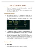
- The histogram is important because if we use an ARMA model for modeling VIX you assume
a normal distribution because you use maximum likelihood.
- In our case is important to note that the series is not normally distributed.
- Formally we can test this by typing sktest VIX
- Skewness should be 0 and kurtosis should be 3 in our case we reject the H0 of normally
distributed variable.
- We already expect this because we saw the histogram.
, 2nd Step – Looking at the autocorrelation plot
Autocorrelation Partial Autocorrelation
1.00
1.00
0.80
Partial autocorrelations of VIX
0.50
0.60
0.40
0.00
0.20
0.00
-0.50
0 10 20 30 40 0 10 20 30 40
Lag Lag
Bartlett's formula for MA(q) 95% confidence bands 95% Confidence bands [se = 1/sqrt(n)]
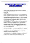
// make a plot of the (partial) autocorrelations
ac VIX in 1/1511, name(ACplot)
pac VIX in 1/1511, name(PACplot)
- We now look at an in-sample period (1511 days)
o You can take also half of the data and test the model on the other half.
What do we see?
- Autocorrelation declines very slowly.
- Partial autocorrelation is almost zero after lag 1 or 2 or 3 .
- This is more AR type of model than MA.
o The reason is because MA says that the autocorrelation will drop immediate to zero
after certain lag. Here it is not the case.
o AR, on the other hand, says that the partial autocorrelation drops to zero and you
can see it in the graph. However, the autocorrelation alone does not decline
exponentially to zero.
- If you see this two plots, you should think that this is more a type of AR MA model but it is
not completely AR therefore we should go for an ARMA model.
, 3rd Step – Estimate ARMA models
//estimate various ARMA models
arima VIX in 1/1511, ar(1/1) ma(1/1)
estat acplot, name(theoACarma11)
arima VIX in 1/1511, ar(1/2) ma(1/1)
estat acplot, name(theoACarma21)
AR(2,1)
ARIMA regression
Sample: 1 - 1511 Number of obs = 1511
Wald chi2(3) = 1.27e+06
Log likelihood = -3068.989 Prob > chi2 = 0.0000
OPG
VIX Coef. Std. Err. z P>|z| [95% Conf. Interval]
VIX
_cons 20.27916 8.485587 2.39 0.017 3.647713 36.9106
ARMA
ar
L1. 1.442787 .0397349 36.31 0.000 1.364908 1.520666
L2. -.4459915 .0392521 -11.36 0.000 -.5229243 -.3690588
ma
L1. -.6463761 .03225 -20.04 0.000 -.709585 -.5831672
/sigma 1.842184 .0119603 154.03 0.000 1.818743 1.865626
Note: The test of the variance against zero is one sided, and the two-sided
confidence interval is truncated at zero.
- Coefficients = 1.44 and -0.44.
- Remember that Ф1 + Ф2 should not exceed 1 here is 0.9967955
Immediately after you estimate the model compute estat ic, n(1511) to look at the AIC and BIC
, - You can’t do anything with the values at the moment because you must compare it with
various models.
AR(1)
- Coefficients = 0.9913489 and -0.2075646.
- Remember that Ф1 + Ф2 should not exceed 1 here is 0.7837843
o This is exactly what we previous thought because the autocorrelations looks almost
like a random walk like an AR1 with the values of 1.
Immediately after you estimate the model compute estat ic, n(1511) to look at the AIC and BIC
, . estat ic, n(1511)
Akaike's information criterion and Bayesian information criterion
Model Obs ll(null) ll(model) df AIC BIC
. 1,511 . -3068.989 5 6147.978 6174.58
Note: N=1511 used in calculating BIC.
- After comparing the AIC and BIC we can conclude that AR (2,1) model has lower values than
AR(1). So, AR(2,1) is better.
- The differences are not that big.
- AR(1) has higher AIC and BIC than AR(2)
o This is because the model look almost like a random walk.
o An AR(1) model with Ф = 0.99 is almost a random walk.
- What you learn from this is that if you see an AC or PAC and you see that is quite close to a
certain model then you already know that if you use other models for forecasting.
4th Step – Construct residuals and check if there is autocorrelation
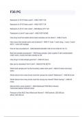
predict resARMA11 in 1/1511, residuals // make residuals
ac resARMA11 in 1/1511, name(ACresARMA11) //plot autocorrelations of the residuals
wntestq resARMA11 in 1/1511, lags(5)
- Until now we estimated the model.
- However, after you do this, you want to check if the model is ok so you check its residuals.
- You create a new variable with the code above.
0.10
0.05
Autocorrelations of AR1
0.00
-0.05
-0.10
0 10 20 30 40
Lag
Bartlett's formula for MA(q) 95% confidence bands
, - You can see that there are 1,970 missing values generated.
- Be careful always to specify you sample in the code.
- This graph does not look good because we see significantly autocorrelation in lag 1, lag 3,
and lag 5.
- Next, we run a test to confirm our outcome
- The F test is very high 41.36, and the p-value is zero.
- We can reject the H0 hypothesis that there is no autocorrelation.
o The test tells us that there is indeed autocorrelation in the residuals.
Conclusion: ARMA (1) has autocorrelation if the residuals. Therefore, let’s look at ARMA (2,1)
AR(2,1)
0.10
Autocorrelations of resARMA12
0.05
0.00
-0.05
-0.10
0 10 20 30 40
Lag
Bartlett's formula for MA(q) 95% confidence bands
- Be careful because you must estimate the model again and change the cod accordingly to fit
with ARMA (2,1)
- The graph looks slightly better than the previous one because I do not see the negative
significant autocorrelation in lag1 anymore.
- We can see something at lag3 and lag 5.
- We run the test again.
, - The F test is also high 27.83, and the p-value is zero but slightly lower than the previous one.
- Also here, we can reject the H0 hypothesis that there is no autocorrelation.
o The test tells us that there is indeed autocorrelation in the residuals.
Conclusion: ARMA (2,1) has autocorrelation if the residuals.
5th Step – Construct the fit of the model
arima VIX in 1/1511, ar(1/1) ma(1/1)
predict fitARMA11 in 1/1511, xb
twoway (line VIX time in 1/1511) (line fitARMA11 time in 1/1511)
AR(1)
80
60
40
20
0
0 500 1000 1500
time
VIX xb prediction, one-step
- The fit of the model looks amazing.
- We see the red line, but we don’t see the blue line anymore.
- The blue line is the original series and the red line is the fit of the 1150 observations.
,AR(2,1)
80
60
40
20
0
0 500 1000 1500
time
VIX xb prediction, one-step
- In terms of fit, we did an extremely good job.
Why does the fit looks so good?
- It is because these time series are full of autocorrelation.
Additional Steps – Test for homoscedasticity
gen res2ARMA11 = resARMA11^2
ac res2ARMA11 in 1/1511, name(ACres2ARMA11)
- We assume from all the ARMA models that the variance of the error terms had a mean of
zero and a variance of σ2 so it is constant.
- You can check whether is true for the VIX while computing the squared residuals (check the
code).
, 0.60
0.40
0.20
0.00
-0.20
0 10 20 30 40
Lag
Bartlett's formula for MA(q) 95% confidence bands
- Huge autocorrelation in squared residuals.
- The squared residuals of today have a lot to do with the squared residuals of yesterday.
- The graph shows that there is heteroscedasticity. The implication of heteroscedasticity is
that is harming the standard error of the coefficients. So, this is bad for the model.
Additional Steps – Log of VIX
- We saw previously that the series was not normally distributed.
- In this case we can compute the log of the VIX
gen lnVIX = ln(VIX)
arima lnVIX in 1/1511, ar(1/1) ma(1/1)
predict ehat_LN_arma11, residuals
gen ehat2_LN_arma11 = ehat_LN_arma11^2
ac ehat2_LN_arma11, name(ACres2ARMA_LOG)
graph combine ACres2ARMA11 ACres2ARMA_LOG
, Autocorrelation Partial Autocorrelation
1.00
1.00
0.80
Partial autocorrelations of VIX
0.50
0.60
0.40
0.00
0.20
0.00
-0.50
0 10 20 30 40 0 10 20 30 40
Lag Lag
Bartlett's formula for MA(q) 95% confidence bands 95% Confidence bands [se = 1/sqrt(n)]
- It looks almost the same at the first ones.
Estimate the model but for the log of the VIX
AR(2,1)
- Coefficients = 1.509166 and -0.5116233
1st Step – Looking to the data
.1
.08
.06
Density
.04
.02
0
0 20 40 60 80
VIX
- The histogram is important because if we use an ARMA model for modeling VIX you assume
a normal distribution because you use maximum likelihood.
- In our case is important to note that the series is not normally distributed.
- Formally we can test this by typing sktest VIX
- Skewness should be 0 and kurtosis should be 3 in our case we reject the H0 of normally
distributed variable.
- We already expect this because we saw the histogram.
, 2nd Step – Looking at the autocorrelation plot
Autocorrelation Partial Autocorrelation
1.00
1.00
0.80
Partial autocorrelations of VIX
0.50
0.60
0.40
0.00
0.20
0.00
-0.50
0 10 20 30 40 0 10 20 30 40
Lag Lag
Bartlett's formula for MA(q) 95% confidence bands 95% Confidence bands [se = 1/sqrt(n)]
// make a plot of the (partial) autocorrelations
ac VIX in 1/1511, name(ACplot)
pac VIX in 1/1511, name(PACplot)
- We now look at an in-sample period (1511 days)
o You can take also half of the data and test the model on the other half.
What do we see?
- Autocorrelation declines very slowly.
- Partial autocorrelation is almost zero after lag 1 or 2 or 3 .
- This is more AR type of model than MA.
o The reason is because MA says that the autocorrelation will drop immediate to zero
after certain lag. Here it is not the case.
o AR, on the other hand, says that the partial autocorrelation drops to zero and you
can see it in the graph. However, the autocorrelation alone does not decline
exponentially to zero.
- If you see this two plots, you should think that this is more a type of AR MA model but it is
not completely AR therefore we should go for an ARMA model.
, 3rd Step – Estimate ARMA models
//estimate various ARMA models
arima VIX in 1/1511, ar(1/1) ma(1/1)
estat acplot, name(theoACarma11)
arima VIX in 1/1511, ar(1/2) ma(1/1)
estat acplot, name(theoACarma21)
AR(2,1)
ARIMA regression
Sample: 1 - 1511 Number of obs = 1511
Wald chi2(3) = 1.27e+06
Log likelihood = -3068.989 Prob > chi2 = 0.0000
OPG
VIX Coef. Std. Err. z P>|z| [95% Conf. Interval]
VIX
_cons 20.27916 8.485587 2.39 0.017 3.647713 36.9106
ARMA
ar
L1. 1.442787 .0397349 36.31 0.000 1.364908 1.520666
L2. -.4459915 .0392521 -11.36 0.000 -.5229243 -.3690588
ma
L1. -.6463761 .03225 -20.04 0.000 -.709585 -.5831672
/sigma 1.842184 .0119603 154.03 0.000 1.818743 1.865626
Note: The test of the variance against zero is one sided, and the two-sided
confidence interval is truncated at zero.
- Coefficients = 1.44 and -0.44.
- Remember that Ф1 + Ф2 should not exceed 1 here is 0.9967955
Immediately after you estimate the model compute estat ic, n(1511) to look at the AIC and BIC
, - You can’t do anything with the values at the moment because you must compare it with
various models.
AR(1)
- Coefficients = 0.9913489 and -0.2075646.
- Remember that Ф1 + Ф2 should not exceed 1 here is 0.7837843
o This is exactly what we previous thought because the autocorrelations looks almost
like a random walk like an AR1 with the values of 1.
Immediately after you estimate the model compute estat ic, n(1511) to look at the AIC and BIC
, . estat ic, n(1511)
Akaike's information criterion and Bayesian information criterion
Model Obs ll(null) ll(model) df AIC BIC
. 1,511 . -3068.989 5 6147.978 6174.58
Note: N=1511 used in calculating BIC.
- After comparing the AIC and BIC we can conclude that AR (2,1) model has lower values than
AR(1). So, AR(2,1) is better.
- The differences are not that big.
- AR(1) has higher AIC and BIC than AR(2)
o This is because the model look almost like a random walk.
o An AR(1) model with Ф = 0.99 is almost a random walk.
- What you learn from this is that if you see an AC or PAC and you see that is quite close to a
certain model then you already know that if you use other models for forecasting.
4th Step – Construct residuals and check if there is autocorrelation
predict resARMA11 in 1/1511, residuals // make residuals
ac resARMA11 in 1/1511, name(ACresARMA11) //plot autocorrelations of the residuals
wntestq resARMA11 in 1/1511, lags(5)
- Until now we estimated the model.
- However, after you do this, you want to check if the model is ok so you check its residuals.
- You create a new variable with the code above.
0.10
0.05
Autocorrelations of AR1
0.00
-0.05
-0.10
0 10 20 30 40
Lag
Bartlett's formula for MA(q) 95% confidence bands
, - You can see that there are 1,970 missing values generated.
- Be careful always to specify you sample in the code.
- This graph does not look good because we see significantly autocorrelation in lag 1, lag 3,
and lag 5.
- Next, we run a test to confirm our outcome
- The F test is very high 41.36, and the p-value is zero.
- We can reject the H0 hypothesis that there is no autocorrelation.
o The test tells us that there is indeed autocorrelation in the residuals.
Conclusion: ARMA (1) has autocorrelation if the residuals. Therefore, let’s look at ARMA (2,1)
AR(2,1)
0.10
Autocorrelations of resARMA12
0.05
0.00
-0.05
-0.10
0 10 20 30 40
Lag
Bartlett's formula for MA(q) 95% confidence bands
- Be careful because you must estimate the model again and change the cod accordingly to fit
with ARMA (2,1)
- The graph looks slightly better than the previous one because I do not see the negative
significant autocorrelation in lag1 anymore.
- We can see something at lag3 and lag 5.
- We run the test again.
, - The F test is also high 27.83, and the p-value is zero but slightly lower than the previous one.
- Also here, we can reject the H0 hypothesis that there is no autocorrelation.
o The test tells us that there is indeed autocorrelation in the residuals.
Conclusion: ARMA (2,1) has autocorrelation if the residuals.
5th Step – Construct the fit of the model
arima VIX in 1/1511, ar(1/1) ma(1/1)
predict fitARMA11 in 1/1511, xb
twoway (line VIX time in 1/1511) (line fitARMA11 time in 1/1511)
AR(1)
80
60
40
20
0
0 500 1000 1500
time
VIX xb prediction, one-step
- The fit of the model looks amazing.
- We see the red line, but we don’t see the blue line anymore.
- The blue line is the original series and the red line is the fit of the 1150 observations.
,AR(2,1)
80
60
40
20
0
0 500 1000 1500
time
VIX xb prediction, one-step
- In terms of fit, we did an extremely good job.
Why does the fit looks so good?
- It is because these time series are full of autocorrelation.
Additional Steps – Test for homoscedasticity
gen res2ARMA11 = resARMA11^2
ac res2ARMA11 in 1/1511, name(ACres2ARMA11)
- We assume from all the ARMA models that the variance of the error terms had a mean of
zero and a variance of σ2 so it is constant.
- You can check whether is true for the VIX while computing the squared residuals (check the
code).
, 0.60
0.40
0.20
0.00
-0.20
0 10 20 30 40
Lag
Bartlett's formula for MA(q) 95% confidence bands
- Huge autocorrelation in squared residuals.
- The squared residuals of today have a lot to do with the squared residuals of yesterday.
- The graph shows that there is heteroscedasticity. The implication of heteroscedasticity is
that is harming the standard error of the coefficients. So, this is bad for the model.
Additional Steps – Log of VIX
- We saw previously that the series was not normally distributed.
- In this case we can compute the log of the VIX
gen lnVIX = ln(VIX)
arima lnVIX in 1/1511, ar(1/1) ma(1/1)
predict ehat_LN_arma11, residuals
gen ehat2_LN_arma11 = ehat_LN_arma11^2
ac ehat2_LN_arma11, name(ACres2ARMA_LOG)
graph combine ACres2ARMA11 ACres2ARMA_LOG
, Autocorrelation Partial Autocorrelation
1.00
1.00
0.80
Partial autocorrelations of VIX
0.50
0.60
0.40
0.00
0.20
0.00
-0.50
0 10 20 30 40 0 10 20 30 40
Lag Lag
Bartlett's formula for MA(q) 95% confidence bands 95% Confidence bands [se = 1/sqrt(n)]
- It looks almost the same at the first ones.
Estimate the model but for the log of the VIX
AR(2,1)
- Coefficients = 1.509166 and -0.5116233