
- Guías de estudio, Notas de estudios & Resúmenes
¿Buscas las mejores guías de estudio, notas de estudio y resúmenes para ? En esta página encontrarás 8 documentos de estudio para .

Examen
AerE 546 Lecture 17 Finite volume method
Finite volume method Natural for unstructured meshed. Also, working with fluxes leads into hyperbolic equations. A. Recall origin of p.d.e.ʼs Donʼt take second step: apply discretization to the integral balance. Control volume is polyline (polyhedron in 3-D). Divergence theorem (Gaussʼ) is used in f.v. method. Rationale: f = ∫df/dx dx but now f ! ∫F·dS and df/dx dx ! ∫ ∇·F dV =∫ ∇·F dS dxn =∫ dF/dxn dxn dS = ∫n·FdS Divergence theorem <-> fundamental theorem...
 Abbyy01

Examen
AerE 546 Lecture 16 (Review finite-diff. and metrics)
Popular(Review finite-diff. and metrics) Second derivatives: Evaluate ∂2ψ/∂2x as ∂xF with F = ∂xψ Outside, then in, but iterated central would give 5 i-points. Wrong: δξ(F) =( Fi+1 - Fi-1 )/2 with F= δξψ → [(ψi+2 -ψi) - (ψi - ψi-2 )]/4. Instead use: ( Fi+1/2 - Fi-1/2 )/2 → [(ψi+1 -ψi) - (ψi - ψi-1 )]/4. Fi+1/2 = value on cell face Fi+1 is data at cell center. Or recall formulating equations in conservation form: Flux in - Flux out + source = rate of change inside c....
Abbyy01

Lote
Aere 546 Lecture 14;15;16;17;18;19;20 Questions And Answers
Algebraic grid generation;(Review finite-diff. and metrics); Equations on curvilinear grids: “metric” tensor; Finite volume method; Hyperbolic Equations; Summary of explicit methods:
Abbyy01
Examen
AerE 546 Lecture 14 Algebraic grid generation
Algebraic grid generation A. A simple, algebraic grid. Grid is a set of points connected by lines (Mesh is the set of points joined into cells.) GRID MESH General idea: mesh surface, propagate into interior -- sometimes by solving elliptic boundary value problem for x(i,j). Choose points on wall, connect them, place tic marks along connecting line = grid; i.e., define surfaces by ( xin(i),yin(i) ) Specify x,y inner and outer then: x(s) = xin + ( xout - xin ) s (0≤ s ≤1) DO i=1,I ...
Abbyy01

Examen
AerE 546 Lecture 15 Equations on curvilinear grids: “metric” tensor
Recall 2-surface method. Grid lines are curved; can use finite diff or finite vol. Former here; will be lectures on latter, but FYI. Actually, grid is a set of points organized into cells. Equations on curvilinear grids: “metric” tensor A. Computational and physical space Grid is not in x-y direction: Grid generation produces [x(i,j),y(i,j)]. Now use that to solve equations. Map from computational to physical. Think of i,j as a grid in ξ - η space. For example δf/δξ = (f(i+1,j...
Abbyy01

Examen
AerE 546 Lecture 18 Hyperbolic Equations
Hyperbolic Equations Physics: Convection and wave propagation; sound in compressible flow. ∂tq = -∇·Fq . Now consider convective (dominated) flux uq. A. Examples: Linearized compressible potential flow (1-M2) ∂x2ϕ + ∂y2ϕ = 0 M>1 is hyperbolic: recall asymptotes=radiation # # # # # c.f. Mach waves Shallow water waves (long waves; non-dispersive): k = 2π/λ; ω = 2π/T ∂t 2h - gH∂x2h = 0 (or ∇2h) ; a = √gH = |ω/k| ; ω = ±k√gH Pictures: expansions and shocks;...
Abbyy01

Examen
AerE 546 Lecture 18 Hyperbolic Equations
Physics: Convection and wave propagation; sound in compressible flow. ∂tq = -∇·Fq . Now consider convective (dominated) flux uq. A. Examples: Linearized compressible potential flow (1-M2) ∂x2ϕ + ∂y2ϕ = 0 M>1 is hyperbolic: recall asymptotes=radiation # # # # # c.f. Mach waves Shallow water waves (long waves; non-dispersive): k = 2π/λ; ω = 2π/T ∂t 2h - gH∂x2h = 0 (or ∇2h) ; a = √gH = |ω/k| ; ω = ±k√gH Pictures: expansions and shocks; .gif animations. Will...
Abbyy01
Examen
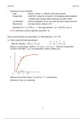
Summary of explicit methods:AerE 546 Lecture 20
Iowa State University AERE 546 Summary of explicit methods: Euler !! upwind = central + ε·diffusion, first order accurate Runge-Kutta !! recall RK is `stable for convectionʼ, time-stepping adds dissipation: ! ! ! variations (low storage, higher damping) are used in CFD. Lax-Wendroff minimum dissipation (ε=C), 2nd order accurate in space and time MacCormick! ! two-step method, similar to L-W Generally CFL < 1, or CFLstab → time-step restriction ∆t < min[ CFLstab ∆x / a NO...
Abbyy01