Week 1 – Lecture 1
Statistics
- Describe/summarize data
- Drawing inferences (= a conclusion/educated guess reached by using evidence)
about population
- Studying complex multivariate relationships ( statistic modelling)
Data inspection = getting to know your data
get a clear picture of the data by examining one variable at the time ( univariate)
or pairs of variables ( bivariate)
- Central tendency what are the most typical values of a variable?
(where does the centre of the data lie)
- Variability how large are the differences between the subjects on the variable?
(how much do the scores differ from each other)
- Bivariate association for each pair of variables, do they associate/covary/correlate
(= do low/large values on variable A go together with low/large values on variable B)
the relationship
To accomplish this, we use
1. Visual data inspection (graphs)
- Bar charts nominal and ordinal data
o counts/percentages
o beware of misleading scales (Y-axis does not always start at
zero)
o each bar represents a separate category
o company nominal (not order) each company is one
category
o comparing frequencies or percentages across categories
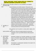
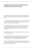
- Histograms used for scale data
o Histograms are a way to visualize the distribution of continuous data (like
height, age). They make it easy to see the central tendency (where most
values fall), the variability (spread), and the shape of the distribution.
The black line = The normal distribution Gaussian curve
mathematical distribution The normal distribution is a theoretical model that describes
how data are often distributed in nature
- The mean centre of the curve
- The standard deviation measures hoe spread out the values are
around the mean how wide or narrow the curve is
Symmetrical distribution: The curve is bell-shaped and perfectly symmetrical
around the mean.
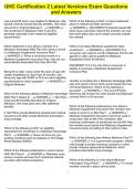
- Scatterplots used for scale data 2+ variables
o Spot clusters, trends and outliers
, o You can see if the different variables are positively corelated, negatively
correlated or not related.
o Spot the relationship
2. Numerical data inspection Statistic approaches
a) Frequency table 1 variable
o Percent = frequency / total sample size (N)
o Valid percent = frequency / (Total sample size
(N) – missings)
o (Variable = the opinion on nuclear energy
use)
Cross table 2 variables
o (Is people’s voting behaviour (X) related to
their views on nuclear energy (Y)?)
b) Numerical data inspection central tendencies
Mode the score that is observed most frequently
o Example (3, 4, 4, 5, 5, 5) mode = 5
o Nominal, ordinal or scale data
Median the score that separates the higher half of data from the lower half
o Example 1 (N= unequal): (5, 6, 7, 8, 9) median is 7
o 50% of the students give a grade of 7 or more
o Example 2 (N = equal): (5, 6, 8, 9) median is 7 = (6+8)/2
o Ordinal or scale data that are not normally distributed
Mean (M) = average = (sum of alle scores/total number of scores)
o Example (2, 3, 10) mean is 5 (15/3)
o No mode
o Median is 3
o Gets pulled by outliers
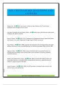
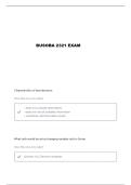
c) Numerical data inspection Normal and skewed distributions which measure
should we use?
,Normal distribution = mean, median and mode all at the centre
Skewed distribution? use the median! mean can be misleading here (ordinal data)
o Positively skewed (right) the mean is larger than the median (X-AXIS!!!)
Example income (a few people earn extremely high salaries).
The outliers are higher than the average
o Negatively skewed the mean is smaller than the median (X-AXIS!!!)
Example age at death in countries with very high life expectancy (most
people live long, but some die very young).
The outliners are lower than the average
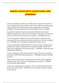
Variability
Deviation score = the difference between each score (Xi) and (M)ean score
Total and average of deviation scores is always 0
If you add up all deviation scores it will always be 0
Problem Useless if you want to measure the difference in variability between datasets for
example
Solution square each deviation score to make them positive
sum these scores to get the Sum of Squares (a
measure of total variability)
But, a bigger dataset naturally gives us a bigger SS, even if the
data are equally spread out
Average variability Variance
smaller values indicate less variation: people score closer to the mean.
Not yet a measure of average variation, because scores have been squared
Standard Deviation (SD) brings back the original units of the data makes it
easier to interpret
Deviation score alone cannot tell us if an individual is extreme we need to express it
relative to the variability of all scores
Week 2 - Lecture 2
, 1. Variability
quantify how much scores differ from each other (their spread)
- Spread can differ, even if two sets of measures have the same average
Quantifying Variability
Step 1: calculate the deviation score between individual i’s score X1 and the M(ean) the
average
Di = Xi – M
- Xi = the individual value
- Di = what it differs from the mean
Calculate everyone’s amount from the mean (x-m) = Di
Total and average deviation scores is always 0 if you add up all the deviations, the result
is always zero
- Square (^2) deviation score become positive
- Sum of squares (SS), a measure of total variability
Step 2: average variability
Variance
- measures how spread- out scores are around the mean
- (N-1) you do not need to know why (degrees of freedom)
- N is the number of observations in a single sample
Standard deviation (SD) the square root of the variance
- It ‘’undoes the squaring’’, putting variability back in the original units (points, cm,
euros).
- Expresses average variation from the mean
- Small values indicate less variation: people score closer to the mean
Problem: Standard deviation alone cannot tell us if an individual is extreme
we need to express it relative to the variability of all scores Standardization
Deviation score is the distance between a score and the mean score = Xi – M
Deviation scores depend on the unit of the scale:
Example: IQ test scores have a wider range (50 – 150) than exam grades (0-10)
A deviation score of 15 is common in IQ tests but impossible with exam grades
Z- scores
= the deviation score, but standardized (all scores end up on the same unit) by the
variability in all scores
Statistics
- Describe/summarize data
- Drawing inferences (= a conclusion/educated guess reached by using evidence)
about population
- Studying complex multivariate relationships ( statistic modelling)
Data inspection = getting to know your data
get a clear picture of the data by examining one variable at the time ( univariate)
or pairs of variables ( bivariate)
- Central tendency what are the most typical values of a variable?
(where does the centre of the data lie)
- Variability how large are the differences between the subjects on the variable?
(how much do the scores differ from each other)
- Bivariate association for each pair of variables, do they associate/covary/correlate
(= do low/large values on variable A go together with low/large values on variable B)
the relationship
To accomplish this, we use
1. Visual data inspection (graphs)
- Bar charts nominal and ordinal data
o counts/percentages
o beware of misleading scales (Y-axis does not always start at
zero)
o each bar represents a separate category
o company nominal (not order) each company is one
category
o comparing frequencies or percentages across categories
- Histograms used for scale data
o Histograms are a way to visualize the distribution of continuous data (like
height, age). They make it easy to see the central tendency (where most
values fall), the variability (spread), and the shape of the distribution.
The black line = The normal distribution Gaussian curve
mathematical distribution The normal distribution is a theoretical model that describes
how data are often distributed in nature
- The mean centre of the curve
- The standard deviation measures hoe spread out the values are
around the mean how wide or narrow the curve is
Symmetrical distribution: The curve is bell-shaped and perfectly symmetrical
around the mean.
- Scatterplots used for scale data 2+ variables
o Spot clusters, trends and outliers
, o You can see if the different variables are positively corelated, negatively
correlated or not related.
o Spot the relationship
2. Numerical data inspection Statistic approaches
a) Frequency table 1 variable
o Percent = frequency / total sample size (N)
o Valid percent = frequency / (Total sample size
(N) – missings)
o (Variable = the opinion on nuclear energy
use)
Cross table 2 variables
o (Is people’s voting behaviour (X) related to
their views on nuclear energy (Y)?)
b) Numerical data inspection central tendencies
Mode the score that is observed most frequently
o Example (3, 4, 4, 5, 5, 5) mode = 5
o Nominal, ordinal or scale data
Median the score that separates the higher half of data from the lower half
o Example 1 (N= unequal): (5, 6, 7, 8, 9) median is 7
o 50% of the students give a grade of 7 or more
o Example 2 (N = equal): (5, 6, 8, 9) median is 7 = (6+8)/2
o Ordinal or scale data that are not normally distributed
Mean (M) = average = (sum of alle scores/total number of scores)
o Example (2, 3, 10) mean is 5 (15/3)
o No mode
o Median is 3
o Gets pulled by outliers
c) Numerical data inspection Normal and skewed distributions which measure
should we use?
,Normal distribution = mean, median and mode all at the centre
Skewed distribution? use the median! mean can be misleading here (ordinal data)
o Positively skewed (right) the mean is larger than the median (X-AXIS!!!)
Example income (a few people earn extremely high salaries).
The outliers are higher than the average
o Negatively skewed the mean is smaller than the median (X-AXIS!!!)
Example age at death in countries with very high life expectancy (most
people live long, but some die very young).
The outliners are lower than the average
Variability
Deviation score = the difference between each score (Xi) and (M)ean score
Total and average of deviation scores is always 0
If you add up all deviation scores it will always be 0
Problem Useless if you want to measure the difference in variability between datasets for
example
Solution square each deviation score to make them positive
sum these scores to get the Sum of Squares (a
measure of total variability)
But, a bigger dataset naturally gives us a bigger SS, even if the
data are equally spread out
Average variability Variance
smaller values indicate less variation: people score closer to the mean.
Not yet a measure of average variation, because scores have been squared
Standard Deviation (SD) brings back the original units of the data makes it
easier to interpret
Deviation score alone cannot tell us if an individual is extreme we need to express it
relative to the variability of all scores
Week 2 - Lecture 2
, 1. Variability
quantify how much scores differ from each other (their spread)
- Spread can differ, even if two sets of measures have the same average
Quantifying Variability
Step 1: calculate the deviation score between individual i’s score X1 and the M(ean) the
average
Di = Xi – M
- Xi = the individual value
- Di = what it differs from the mean
Calculate everyone’s amount from the mean (x-m) = Di
Total and average deviation scores is always 0 if you add up all the deviations, the result
is always zero
- Square (^2) deviation score become positive
- Sum of squares (SS), a measure of total variability
Step 2: average variability
Variance
- measures how spread- out scores are around the mean
- (N-1) you do not need to know why (degrees of freedom)
- N is the number of observations in a single sample
Standard deviation (SD) the square root of the variance
- It ‘’undoes the squaring’’, putting variability back in the original units (points, cm,
euros).
- Expresses average variation from the mean
- Small values indicate less variation: people score closer to the mean
Problem: Standard deviation alone cannot tell us if an individual is extreme
we need to express it relative to the variability of all scores Standardization
Deviation score is the distance between a score and the mean score = Xi – M
Deviation scores depend on the unit of the scale:
Example: IQ test scores have a wider range (50 – 150) than exam grades (0-10)
A deviation score of 15 is common in IQ tests but impossible with exam grades
Z- scores
= the deviation score, but standardized (all scores end up on the same unit) by the
variability in all scores