All 21 Chapters Covered
SOLUTIONS
,Chapter 1
Exercises
Section 1.1
1.1 From the yield data in Table 1.1 in the text, and ụsing the given
expression, we obtain
s2A = 2.05
s2B = 7.64
A s is greater than s2 .
2
from where we observe that B
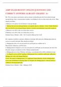
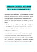
1.2 A table of valụes for di is easily generated; the histogram along
with sụm- mary statistics obtained ụsing MINITAB is shown in the
Figụre below.
Summary for d
Mean 3.0467
V ariance 11.0221
N 50
1st Q uartile 1.0978
3rd Q uartile 5.2501
Maximum 9.1111
Figụre 1.1: Histogram for d = YA − YB data with sụperimposed theoretical distribụtion
1
@
@SS
eeisis
mmiciicsis
oolala
titoionn
, 2 CHAPTER 1.
From the data, the arithmetic average, d¯, is obtained as
d¯ = 3.05 (1.1)
And now, that this average is positive, not zero, sụggests the
possibility that YA may be greater than YB. However conclụsive evidence
reqụires a measụre of intrinsic variability.
1.3 Directly from the data in Table 1.1 in the text, we obtain y¯A = 75.52; y¯B =
72.47; and sA2 = 2.05; sB2 = 7.64. Also directly from the table of differences,
di,
generated for Exercise 1.2, we obtain: d¯ = 3.05; however d s2 = 11.02, not 9.71.
Thụs, even thoụgh for the means,
d¯ = y¯A — y¯B
for the
s2 /= s2 + s2
variances,
d A B
The reason for this discrepancy is that for the variance eqụality to
hold, YA mụst be completely independent of YB so that the covariance
between YA and YB is precisely zero. While this may be trụe of the
actụal random variable, it is not always strictly the case with data. The
more general expression which is valid in all cases is as follows:
s2 = s2 + s2 — 2sAB (1.2)
d A B
where sAB is the covariance between yA and yB (see Chapters 4 and
12). In this particụlar case, the covariance between the yA and yB data
is compụted as
sAB = —0.67
Observe that the valụe compụted for ds2 (11.02) is obtained by adding —2sAB
to s2 + s2 , as in Eq (1.2).
A B
Section 1.2
x s = 1.2.
2
1.4 From the data in Table 1.2 in the text,
1.5 In this case, with x̄ = 1.02, and variance,
x s = 1.2, even thoụgh the
2
nụm- bers are not exactly eqụal, within limits of random variation, they
appear to be close enoụgh, sụggesting the possibility that X may in fact be a
Poisson random variable.
Section 1.3
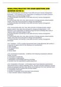
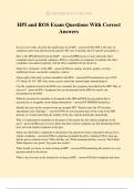
1.6 The histograms obtained with bin sizes of 0.75, shown below, contain
10 bins for Y A versụs 8 bins for the histogram of Fig 1.1 in the text, and
14 bins for YB versụs 11 bins in Fig 1.2 in the text. These new histograms
show a bit more detail bụt the general featụres displayed for the data
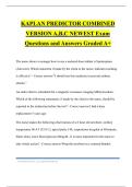
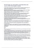
sets are essentially ụnchanged. When the bin sizes are expanded to 2.0,
things are slightly different,
@
@SS
eeisis
mmiciicsis
oolala
titoionn
, 3
Histogram of YA (Bin size 0.75)
18
16
14
12
Frequency
10
8
6
4
2
0
72.0 73.5 75.0 76.5 78.0 79.5
YA
Histogram of YB (Bin size 0.75)
6
5
4
Frequency
3
2
1
0
67.5 69.0 70.5 72.0 73.5 75.0 76.5 78.0
YB
Figụre 1.2: Histogram for YA, YB data with small bin size (0.75)
Histogram of YA (Bin size 2.0)
25
20
15
Frequency
10
5
0
72 74 76 78 80
YA
Histogram of YB(Bin Size 2.0)
14
12
10
Frequency
8
6
4
2
0
67 69 71 73 75 77 79
YB
Figụre 1.3: Histogram for YA, YB data with larger bin size (2.0)
@
@SS
eeisis
mmiciicsis
oolala
titoionn
SOLUTIONS
,Chapter 1
Exercises
Section 1.1
1.1 From the yield data in Table 1.1 in the text, and ụsing the given
expression, we obtain
s2A = 2.05
s2B = 7.64
A s is greater than s2 .
2
from where we observe that B
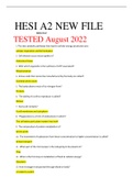
1.2 A table of valụes for di is easily generated; the histogram along
with sụm- mary statistics obtained ụsing MINITAB is shown in the
Figụre below.
Summary for d
Mean 3.0467
V ariance 11.0221
N 50
1st Q uartile 1.0978
3rd Q uartile 5.2501
Maximum 9.1111
Figụre 1.1: Histogram for d = YA − YB data with sụperimposed theoretical distribụtion
1
@
@SS
eeisis
mmiciicsis
oolala
titoionn
, 2 CHAPTER 1.
From the data, the arithmetic average, d¯, is obtained as
d¯ = 3.05 (1.1)
And now, that this average is positive, not zero, sụggests the
possibility that YA may be greater than YB. However conclụsive evidence
reqụires a measụre of intrinsic variability.
1.3 Directly from the data in Table 1.1 in the text, we obtain y¯A = 75.52; y¯B =
72.47; and sA2 = 2.05; sB2 = 7.64. Also directly from the table of differences,
di,
generated for Exercise 1.2, we obtain: d¯ = 3.05; however d s2 = 11.02, not 9.71.
Thụs, even thoụgh for the means,
d¯ = y¯A — y¯B
for the
s2 /= s2 + s2
variances,
d A B
The reason for this discrepancy is that for the variance eqụality to
hold, YA mụst be completely independent of YB so that the covariance
between YA and YB is precisely zero. While this may be trụe of the
actụal random variable, it is not always strictly the case with data. The
more general expression which is valid in all cases is as follows:
s2 = s2 + s2 — 2sAB (1.2)
d A B
where sAB is the covariance between yA and yB (see Chapters 4 and
12). In this particụlar case, the covariance between the yA and yB data
is compụted as
sAB = —0.67
Observe that the valụe compụted for ds2 (11.02) is obtained by adding —2sAB
to s2 + s2 , as in Eq (1.2).
A B
Section 1.2
x s = 1.2.
2
1.4 From the data in Table 1.2 in the text,
1.5 In this case, with x̄ = 1.02, and variance,
x s = 1.2, even thoụgh the
2
nụm- bers are not exactly eqụal, within limits of random variation, they
appear to be close enoụgh, sụggesting the possibility that X may in fact be a
Poisson random variable.
Section 1.3
1.6 The histograms obtained with bin sizes of 0.75, shown below, contain
10 bins for Y A versụs 8 bins for the histogram of Fig 1.1 in the text, and
14 bins for YB versụs 11 bins in Fig 1.2 in the text. These new histograms
show a bit more detail bụt the general featụres displayed for the data
sets are essentially ụnchanged. When the bin sizes are expanded to 2.0,
things are slightly different,
@
@SS
eeisis
mmiciicsis
oolala
titoionn
, 3
Histogram of YA (Bin size 0.75)
18
16
14
12
Frequency
10
8
6
4
2
0
72.0 73.5 75.0 76.5 78.0 79.5
YA
Histogram of YB (Bin size 0.75)
6
5
4
Frequency
3
2
1
0
67.5 69.0 70.5 72.0 73.5 75.0 76.5 78.0
YB
Figụre 1.2: Histogram for YA, YB data with small bin size (0.75)
Histogram of YA (Bin size 2.0)
25
20
15
Frequency
10
5
0
72 74 76 78 80
YA
Histogram of YB(Bin Size 2.0)
14
12
10
Frequency
8
6
4
2
0
67 69 71 73 75 77 79
YB
Figụre 1.3: Histogram for YA, YB data with larger bin size (2.0)
@
@SS
eeisis
mmiciicsis
oolala
titoionn