BRM
BRUSHING UP
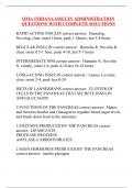
watched reviewed duration topic
31 min Hypothesis testing
1 h 16 Linear regression
25 min SPSS
LOGISTIC REGRESSION
watched reviewed duration topic
1 h 24 Logistic regression (I)
41 min Logistic regression (II)
40 min Logistic regression (III)
23 min Logistic regression (IV)
22 min Logistic regression (example)
23 min Logistic regression (ex.3)
Exercises: 1 – 2 – 3 – 4 – 5 – 6
FACTOR ANALYSIS
watched reviewed duration topic
1 h 16 Factor analysis (I)
30 min Factor analysis (II)
16 min Factor analysis (example)
19 min Factor analysis (SPSS)
Exercises: 1 – 2 – 3 – 4 – 5 –
RELIABILITY ANALYSIS
watched reviewed duration topic
34 min Reliability analysis
22 min Reliability analysis (SPSS)
CLUSTER ANALYSIS
watched reviewed duration topic
1h 18 Cluster analysis
10 min Cluster analysis (SPSS)
Exercises: 1 – 2 – 3 – 4 – 5
SYNTHESIS EXERCISE
watched reviewed duration topic
39 min Synthesis exercise
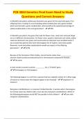
,Formula sheet BRM Factoranalysis
Logistic regression Factor model:
Model: 1 Xi = ai1 F1 + ai2 F2 + …+ aik Fk + Ui
P (Y = 1) = Fj = wj1 X1 + wj2 X2 + …+ wjp Xp
1 + exp(−(α + β1 x1 + β 2 x2 + ... + β p x p ))
k k
=
exp(α + β1 x1 + β 2 x2 + ... + β p x p ) ∑∑
i =1 j =1,i ≠ j
rij2
1 + exp(α + β1 x1 + β 2 x2 + ... + β p x p ) Kaiser-Meyer-Olkin : KMO = k k k k
Odds = P(Y=1) / P(Y=0) ∑∑
i =1 j =1,i ≠ j
2
ijr +∑ ∑a
i =1 j =1,i ≠ j
2
ij
Likelihood Ratio Test:
- Comparing Model 1 with Model 2, for which Model 1 is Kaiser-Meyer-Olkin for individual variable:
k
∑
nested in Model 2
- H0 : all coeff of extra variables in Model 2 are equal to 0 rij2
j =1,i ≠ j
- Test statistic = Likelihood Ratio (LR) KMOi = k k
= (-2LogLik(Model 1)) – (-2LogLik(Model 2))
- Under H0 LR has a chi-squared distribution with k degrees of ∑r
j =1,i ≠ j
2
ij + ∑a
j =1,i ≠ j
2
ij
freedom, for which k is the number of extra parameters that
are estimated in Model 2.
%&' ,
Fraction of the total variance explained by the first k (of p) factors (for
Wald test: H0: βi = 0, Wald-statistic: " = $ + ~ χ., λ1 + λ2 + L + λk
()*
PCA) =
Confidence interval for a coefficient β = b ± z* SEB p
Specificity = % of correct classifications of Y=0 2 2 2
Sensitivity = % of correct classifications of Y=1 Communality of the i-th variable = ai1 + ai 2 + L + aik
/01 23/0&2345 23/0
Standardized residual = Fraction of the total variance explained by factor j
62345 23/0 (.&2345 23/0)
Hosmer and Lemeshow test: H0: no difference between observed ( 2 2
= a1 j + a2 j + L + a pj / p
2
)
and predicted probabilities Reproduced correlation between variable i and j:
QMC when tolerance < 0.2 or VIF>5 rˆij = ai1a j1 + ai 2 a j 2 + L + aik a jk
Residual = rij − rˆij
Clusteranalysis
d ²( A, B) = ∑ ( xk , A − xk , B )
2
Squared Euclidian distance : Cronbach’s Alpha
k ∑
k
Var(itemi )
Single linkage = nearest neighbour
α= 1− i
Complete linkage = furthest neighbour
k −1 Var(scale)
UPGMA = Average linkage of between-group linkage
, BRM – Logistic regression
1. The logistic regression model
• Dependent variable Y = a binary/dichotomous/dummy variable (0/1).
• Directly estimate the probability that one of two events occur, based on a set of independent variables that can
be either quantitative or dummy variables.
• We usually estimate the probability that Y = 1.
• When you set a categorical variable with more than two categories, you have to create (n-1) dummies with one
reference group.
Why not a classical linear regression?
• Not a linear relation needed.
• Only results: 0-1.
• Thus, a classical linear regression is not optimal for a dependent variable that is binary.
General logistic regression model
• Given: Y is a binary dependent variable.
• Given: X1, X2, X…, Xp: explanatory variables, which can be either quantitative or dummy variables.
• Formula: first one on formula sheet.
Dummies
• SPSS
• (n-1) dummies with one reference category: usually first or last. Automatically done, but can be changed.
2. Regression coefficients
Estimation method
• Loglikelihood = measures how likely the observations are under the model. A high loglikelihood indicates a good
model.
• Remark: the more data, the better. You need at least 10 Y=1 (event) and Y=0 (non event) for every variable in
the model.
Interpretation in terms of probabilities
• Fill in values in formula or let SPSS do it.
• “The probability that Y=1, is estimated as …”
Interpretation in terms of odds
• Odds: ratio of the probability that an event occurs to the probability that it does not occur.
o Odds = 1: it is as likely that the event occurs (Y=1), than that it does not occur (Y=0).
o Odds < 1: it is less probable that the event occurs (Y=1), than that it does not occur (Y=0).
o Odds > 1: it is more probable that the event occurs (Y=1), than that it does not occur (Y=0).
• Odds ratio: ratio of two odds to compare two groups.
o Bi = 0 and odds ratio Exp(Bi) = 1: the ith variable has no effect on the response.
o Bi < 0 and odds ratio Exp(Bi) < 1: the ith variable has a negative effect on the response (the odds of the
event are decreased).
o Bi > 0 and odds ratio Exp(Bi) > 1: the ith variable has a positive effect on the response (the odds of the
event are increased).
• For categorical variables with more than two answers: the reference category should be used for comparison.
, Example
• Y=1 lymph nodes are cancerous and Y=0 otherwise.
• Continuous variables:
o acid
§ B = 0.024: > 0 and Exp(B) = 1.025: odds ratio > 1
§ The odds of cancerous nodes change with a factor 1.025 if acid rises with 1 unit, ceteris paribus.
Therefore, acid has a positive effect on the fact that nodes are cancerous.
o age
§ B = -0.069: < 0 and Exp(B) = 0.933: odds ratio < 1
§ The odds of cancerous nodes change with a factor 0.933 if age rises with 1 unit, ceteris paribus.
Therefore, age has a negative effect on the fact that nodes are cancerous.
• Categorical variables (dummies):
o xray
§ B = 2.045: > 0 and Exp(B) = 7.732: odds ratio > 1
§ The odds of cancerous nodes when someone has a positive x-ray result (xray = 1) is 7.732
times larger than the odds of cancerous nodes for someone who has a negative x-ray result
(xray = 0), ceteris paribus.
o stage
§ B = 1.564: > 0 and Exp(B) = 4.778: odds ratio > 1
§ The odds of cancerous nodes when someone is in an advanced stage of cancer (stage = 1) is
4.778 times larger than the odds of cancerous nodes for someone who is not in an advanced
stage of cancer (stage = 0), ceteris paribus.
o grade
§ B = 0.761: > 0 and Exp(B) = 2.1: odds ratio > 1
§ The odds of cancerous nodes when someone has an aggressively spread tumor (grade = 1) is
2.1 times larger than the odds of cancerous nodes for someone who has no aggressively
spread tumor (grade = 0), ceteris paribus.
3. Testing hypotheses about the model
Testing whether we have a useful model
• Likelihood ratio test (remember for linear regression: F-test)
• R2: be careful with the interpretation
Testing whether we have significant variables
• Wald test
• Likelihood ratio test
Likelihood ratio test: do we have a useful model? And, do we have significant variables?
• In general: full model versus reduced model.
• The higher the likelihood of a model, the better.
• The likelihood rises when extra variables are added to the model (cfr. R2 rises in linear regression). But is this
rise significant?
• Advantage: better results (vs Wald Test)
• Disadvantage: computationally more intensive (vs Wald Test)
, • The test statistic compares the likelihood of the full model with the likelihood of the reduced model:
o TS = -2 Log Lreduced – (-2 Log Lfull)
o TS ≈ Xk2 with k = difference between the number of parameters in the two models (if n large enough
and no (or very few) continuous variables in the model).
• Remark: only use models that are nested.
• Useful model?
o H0: all Bi = 0
o H1: there is a Bi ≠ 0
o We want to be able to reject H0, for a p-value < 0.05.
• The test statistic compares the likelihood of the model with the likelihood of the model that contains only the
intercept:
o TS = -2 Log Lint – (-2 Log Lmodel)
o TS ≈ Xp2
Example
• Block 0
• Block 1
• Steps:
o Block 0:
§ results of the reduced model
§ -2 Log Likelihood = 70.252
o Block 1:
§ results of the full model
§ -2 Log Likelihood = 48.126
o Test statistic:
§ Formula: -2 Log Lint – (-2 Log Lmodel) = 70.252 – 48.126 = 22.126
o Usueful model:
§ Look at Omnibus Test output: Model line: p-value = 0 < 0.05: we reject H0, meaning we have a
useful model.
§ Look at Omnibus Test output: Block line: p-value = 0 < 0.05: we reject H0, meaning at least one
variable in the model is significant
o Remark: do not delete all ‘non-significant’ variables from your model after the enter-method. It is also
interesting to see that a variable is not significant.
BRUSHING UP
watched reviewed duration topic
31 min Hypothesis testing
1 h 16 Linear regression
25 min SPSS
LOGISTIC REGRESSION
watched reviewed duration topic
1 h 24 Logistic regression (I)
41 min Logistic regression (II)
40 min Logistic regression (III)
23 min Logistic regression (IV)
22 min Logistic regression (example)
23 min Logistic regression (ex.3)
Exercises: 1 – 2 – 3 – 4 – 5 – 6
FACTOR ANALYSIS
watched reviewed duration topic
1 h 16 Factor analysis (I)
30 min Factor analysis (II)
16 min Factor analysis (example)
19 min Factor analysis (SPSS)
Exercises: 1 – 2 – 3 – 4 – 5 –
RELIABILITY ANALYSIS
watched reviewed duration topic
34 min Reliability analysis
22 min Reliability analysis (SPSS)
CLUSTER ANALYSIS
watched reviewed duration topic
1h 18 Cluster analysis
10 min Cluster analysis (SPSS)
Exercises: 1 – 2 – 3 – 4 – 5
SYNTHESIS EXERCISE
watched reviewed duration topic
39 min Synthesis exercise
,Formula sheet BRM Factoranalysis
Logistic regression Factor model:
Model: 1 Xi = ai1 F1 + ai2 F2 + …+ aik Fk + Ui
P (Y = 1) = Fj = wj1 X1 + wj2 X2 + …+ wjp Xp
1 + exp(−(α + β1 x1 + β 2 x2 + ... + β p x p ))
k k
=
exp(α + β1 x1 + β 2 x2 + ... + β p x p ) ∑∑
i =1 j =1,i ≠ j
rij2
1 + exp(α + β1 x1 + β 2 x2 + ... + β p x p ) Kaiser-Meyer-Olkin : KMO = k k k k
Odds = P(Y=1) / P(Y=0) ∑∑
i =1 j =1,i ≠ j
2
ijr +∑ ∑a
i =1 j =1,i ≠ j
2
ij
Likelihood Ratio Test:
- Comparing Model 1 with Model 2, for which Model 1 is Kaiser-Meyer-Olkin for individual variable:
k
∑
nested in Model 2
- H0 : all coeff of extra variables in Model 2 are equal to 0 rij2
j =1,i ≠ j
- Test statistic = Likelihood Ratio (LR) KMOi = k k
= (-2LogLik(Model 1)) – (-2LogLik(Model 2))
- Under H0 LR has a chi-squared distribution with k degrees of ∑r
j =1,i ≠ j
2
ij + ∑a
j =1,i ≠ j
2
ij
freedom, for which k is the number of extra parameters that
are estimated in Model 2.
%&' ,
Fraction of the total variance explained by the first k (of p) factors (for
Wald test: H0: βi = 0, Wald-statistic: " = $ + ~ χ., λ1 + λ2 + L + λk
()*
PCA) =
Confidence interval for a coefficient β = b ± z* SEB p
Specificity = % of correct classifications of Y=0 2 2 2
Sensitivity = % of correct classifications of Y=1 Communality of the i-th variable = ai1 + ai 2 + L + aik
/01 23/0&2345 23/0
Standardized residual = Fraction of the total variance explained by factor j
62345 23/0 (.&2345 23/0)
Hosmer and Lemeshow test: H0: no difference between observed ( 2 2
= a1 j + a2 j + L + a pj / p
2
)
and predicted probabilities Reproduced correlation between variable i and j:
QMC when tolerance < 0.2 or VIF>5 rˆij = ai1a j1 + ai 2 a j 2 + L + aik a jk
Residual = rij − rˆij
Clusteranalysis
d ²( A, B) = ∑ ( xk , A − xk , B )
2
Squared Euclidian distance : Cronbach’s Alpha
k ∑
k
Var(itemi )
Single linkage = nearest neighbour
α= 1− i
Complete linkage = furthest neighbour
k −1 Var(scale)
UPGMA = Average linkage of between-group linkage
, BRM – Logistic regression
1. The logistic regression model
• Dependent variable Y = a binary/dichotomous/dummy variable (0/1).
• Directly estimate the probability that one of two events occur, based on a set of independent variables that can
be either quantitative or dummy variables.
• We usually estimate the probability that Y = 1.
• When you set a categorical variable with more than two categories, you have to create (n-1) dummies with one
reference group.
Why not a classical linear regression?
• Not a linear relation needed.
• Only results: 0-1.
• Thus, a classical linear regression is not optimal for a dependent variable that is binary.
General logistic regression model
• Given: Y is a binary dependent variable.
• Given: X1, X2, X…, Xp: explanatory variables, which can be either quantitative or dummy variables.
• Formula: first one on formula sheet.
Dummies
• SPSS
• (n-1) dummies with one reference category: usually first or last. Automatically done, but can be changed.
2. Regression coefficients
Estimation method
• Loglikelihood = measures how likely the observations are under the model. A high loglikelihood indicates a good
model.
• Remark: the more data, the better. You need at least 10 Y=1 (event) and Y=0 (non event) for every variable in
the model.
Interpretation in terms of probabilities
• Fill in values in formula or let SPSS do it.
• “The probability that Y=1, is estimated as …”
Interpretation in terms of odds
• Odds: ratio of the probability that an event occurs to the probability that it does not occur.
o Odds = 1: it is as likely that the event occurs (Y=1), than that it does not occur (Y=0).
o Odds < 1: it is less probable that the event occurs (Y=1), than that it does not occur (Y=0).
o Odds > 1: it is more probable that the event occurs (Y=1), than that it does not occur (Y=0).
• Odds ratio: ratio of two odds to compare two groups.
o Bi = 0 and odds ratio Exp(Bi) = 1: the ith variable has no effect on the response.
o Bi < 0 and odds ratio Exp(Bi) < 1: the ith variable has a negative effect on the response (the odds of the
event are decreased).
o Bi > 0 and odds ratio Exp(Bi) > 1: the ith variable has a positive effect on the response (the odds of the
event are increased).
• For categorical variables with more than two answers: the reference category should be used for comparison.
, Example
• Y=1 lymph nodes are cancerous and Y=0 otherwise.
• Continuous variables:
o acid
§ B = 0.024: > 0 and Exp(B) = 1.025: odds ratio > 1
§ The odds of cancerous nodes change with a factor 1.025 if acid rises with 1 unit, ceteris paribus.
Therefore, acid has a positive effect on the fact that nodes are cancerous.
o age
§ B = -0.069: < 0 and Exp(B) = 0.933: odds ratio < 1
§ The odds of cancerous nodes change with a factor 0.933 if age rises with 1 unit, ceteris paribus.
Therefore, age has a negative effect on the fact that nodes are cancerous.
• Categorical variables (dummies):
o xray
§ B = 2.045: > 0 and Exp(B) = 7.732: odds ratio > 1
§ The odds of cancerous nodes when someone has a positive x-ray result (xray = 1) is 7.732
times larger than the odds of cancerous nodes for someone who has a negative x-ray result
(xray = 0), ceteris paribus.
o stage
§ B = 1.564: > 0 and Exp(B) = 4.778: odds ratio > 1
§ The odds of cancerous nodes when someone is in an advanced stage of cancer (stage = 1) is
4.778 times larger than the odds of cancerous nodes for someone who is not in an advanced
stage of cancer (stage = 0), ceteris paribus.
o grade
§ B = 0.761: > 0 and Exp(B) = 2.1: odds ratio > 1
§ The odds of cancerous nodes when someone has an aggressively spread tumor (grade = 1) is
2.1 times larger than the odds of cancerous nodes for someone who has no aggressively
spread tumor (grade = 0), ceteris paribus.
3. Testing hypotheses about the model
Testing whether we have a useful model
• Likelihood ratio test (remember for linear regression: F-test)
• R2: be careful with the interpretation
Testing whether we have significant variables
• Wald test
• Likelihood ratio test
Likelihood ratio test: do we have a useful model? And, do we have significant variables?
• In general: full model versus reduced model.
• The higher the likelihood of a model, the better.
• The likelihood rises when extra variables are added to the model (cfr. R2 rises in linear regression). But is this
rise significant?
• Advantage: better results (vs Wald Test)
• Disadvantage: computationally more intensive (vs Wald Test)
, • The test statistic compares the likelihood of the full model with the likelihood of the reduced model:
o TS = -2 Log Lreduced – (-2 Log Lfull)
o TS ≈ Xk2 with k = difference between the number of parameters in the two models (if n large enough
and no (or very few) continuous variables in the model).
• Remark: only use models that are nested.
• Useful model?
o H0: all Bi = 0
o H1: there is a Bi ≠ 0
o We want to be able to reject H0, for a p-value < 0.05.
• The test statistic compares the likelihood of the model with the likelihood of the model that contains only the
intercept:
o TS = -2 Log Lint – (-2 Log Lmodel)
o TS ≈ Xp2
Example
• Block 0
• Block 1
• Steps:
o Block 0:
§ results of the reduced model
§ -2 Log Likelihood = 70.252
o Block 1:
§ results of the full model
§ -2 Log Likelihood = 48.126
o Test statistic:
§ Formula: -2 Log Lint – (-2 Log Lmodel) = 70.252 – 48.126 = 22.126
o Usueful model:
§ Look at Omnibus Test output: Model line: p-value = 0 < 0.05: we reject H0, meaning we have a
useful model.
§ Look at Omnibus Test output: Block line: p-value = 0 < 0.05: we reject H0, meaning at least one
variable in the model is significant
o Remark: do not delete all ‘non-significant’ variables from your model after the enter-method. It is also
interesting to see that a variable is not significant.