,Contents
1 The Postulates of Quantum Mechanics ................................................ 1
1.1 Quantum States .......................................................................... 2
1.1.1 Pure States ....................................................................... 2
1.1.2 Mixed States ..................................................................... 7
1.2 Time Evolution of Quantum States ............................................. 16
1.2.1 Unitary Dynamics............................................................ 17
1.2.2 Quantum Noisy Dynamics ............................................... 20
1.3 Measurements on Quantum States ............................................ 21
1.3.1 Projection Measurements ................................................ 21
1.3.2 Generalized Measurements............................................. 26
2 Quantum Computation: Overview ...................................................... 33
2.1 Single-Qubit Gates .................................................................... 34
2.1.1 Pauli Gates ..................................................................... 34
2.1.2 Hadamard Gate .............................................................. 39
2.1.3 Rotations ........................................................................ 42
2.2 Two-Qubit Gates ....................................................................... 46
2.2.1 CNOT, CZ, and SWAP................................................................ 46
2.2.2 Controlled-Unitary Gate................................................... 57
2.2.3 General Unitary Gate ...................................................... 63
2.3 Multi-Qubit Controlled Gates...................................................... 70
2.3.1 Gray Code ...................................................................... 71
2.3.2 Multi-Qubit Controlled-NOT ............................................. 73
2.4 Universal Quantum Computation ............................................... 79
2.5 Measurements .......................................................................... 81
3 Realizations of Quantum Computers 89
.3.1. . . . Quantum
. . . . . . . . . Bits
. . . . ...................... . . . . . . . . . . . . . . . . . . . . . . . . . . . . . . . 90
.3.2
. . . Dynamical Scheme . . . . . . . . . . . . . . . . . . . . . . . . . . . . . . . . . . . . . 92
. . . . 3.2.1 Implementation of Single-Qubit Gates . . . . . . . . . . . . . . . 93
.3.2.2
.. Implementation of CNOT . 99
............................
vii
,viii Contents
3.3 Geometric/Topological Scheme.................................................102
3.3.1 A Toy Model ...................................................................103
3.3.2 Geometric Phase ...........................................................109
3.4 Measurement-Based Scheme...................................................112
3.4.1 Single-Qubit Rotations ...................................................116
3.4.2 CNOT Gate ....................................................................119
3.4.3 Graph States..................................................................122
4 Quantum Algorithms.........................................................................127
4.1 Quantum Teleportation .............................................................128
4.1.1 Nonlocality in Entanglement ...........................................129
4.1.2 Implementation of Quantum Teleportation .......................132
4.2 Deutsch-Jozsa Algorithm & Variants ............................................. 136
4.2.1 Quantum Oracle.............................................................136
4.2.2 Deutsch-Jozsa Algorithm................................................142
4.2.3 Bernstein-Vazirani Algorithm ..........................................144
4.2.4 Simon’s Algorithm ..........................................................145
4.3 Quantum Fourier Transform (QFT) .......................................... 150
4.3.1 Definition and Physical Meaning .....................................150
4.3.2 Quantum Implementation ...............................................152
4.3.3 Semiclassical Implementation.........................................156
4.4 Quantum Phase Estimation (QPE) ............................................160
4.4.1 Definition........................................................................160
4.4.2 Implementation ..............................................................162
4.4.3 Accuracy ........................................................................165
4.4.4 Simulation of the von Neumann Measurement ................166
4.5 Applications..............................................................................167
4.5.1 The Period-Finding Algorithm .........................................168
4.5.2 The Order-Finding Algorithm ..........................................175
4.5.3 Quantum Factorization Algorithm ....................................177
4.5.4 Quantum Search Algorithm ............................................178
5 Quantum Decoherence.....................................................................189
5.1 How Does Decoherence Occur? ...............................................190
5.2 Quantum Operations ................................................................196
5.2.1 Kraus Representation.....................................................197
5.2.2 Choi Isomorphism ..........................................................206
5.2.3 Unitary Representation ...................................................209
5.2.4 Examples .......................................................................210
5.3 Measurements as Quantum Operations ....................................215
5.4 Quantum Master Equation ........................................................216
5.4.1 Derivation.......................................................................219
5.4.2 Examples .......................................................................220
5.4.3 Solution Methods ...........................................................223
5.4.4 Examples Revisited........................................................229
Contents ix
, 5.5 Distance Between Quantum States ...........................................234
5.5.1 Norms and Distances .....................................................234
5.5.2 Hilbert–Schmidt and Trace Norms ...................................236
5.5.3 Hilbert–Schmidt and Trace Distances ..............................241
5.5.4 Fidelity .......................................................................... 246
6 Quantum Error-Correction Codes......................................................257
6.1 Elementary Examples: Nine-Qubit Code ...................................258
6.1.1 Bit-Flip Errors .................................................................258
6.1.2 Phase-Flip Error............................................................ 261
6.1.3 Shor’s Nine-Qubit Code ..................................................263
6.2 Quantum Error Correction.........................................................268
6.2.1 Quantum Error-Correction Conditions .............................268
6.2.2 Discretization of Errors ...................................................270
6.3 Stabilizer Formalism .................................................................271
6.3.1 Pauli Group ....................................................................274
6.3.2 Properties of the Stabilizers ........................................... 279
6.3.3 Unitary Gates in Stabilizer Formalism .............................282
6.3.4 Clifford Group.................................................................283
6.3.5 Measurements in Stabilizer Formalism .......................... 290
6.3.6 Examples .......................................................................291
6.4 Stabilizer Codes .......................................................................297
6.4.1 Bit-Flip Code ..................................................................299
6.4.2 Phase-Flip Code ............................................................301
6.4.3 Nine-Qubit Code ............................................................302
6.4.4 Five-Qubit Code .............................................................305
6.5 Surface Codes .........................................................................309
6.5.1 Toric Codes....................................................................310
6.5.2 Planar Codes .................................................................314
6.5.3 Recovery Procedure.......................................................316
7 Quantum Information Theory ............................................................323
7.1 Shannon Entropy......................................................................324
7.1.1 Definition........................................................................324
7.1.2 Relative Entropy .............................................................326
7.1.3 Mutual Information .........................................................328
7.1.4 Data Compression .........................................................330
7.2 Von Neumann Entropy ..............................................................331
7.2.1 Definition........................................................................331
7.2.2 Relative Entropy .............................................................334
7.2.3 Quantum Mutual Information ..........................................337
7.3 Entanglement and Entropy........................................................338
7.3.1 What is Entanglement? ..................................................339
7.3.2 Separability Tests ............................................................... 339
7.3.3 Entanglement Distillation ............................................... 343
7.3.4 Entanglement Measures.................................................345
x Contents
,Appendix A: Linear Algebra ................................................................. 349
Appendix B: Superoperators................................................................... 373
Appendix C: Group Theory..................................................................... 395
Appendix D: Mathematica Application Q3 ............................................... 405
Appendix E: Integrated Compilation of Demonstrations ........................... 407
Appendix F: Solutions to Select Problems............................................... 409
Bibliography .................................................................................................... 425
Index............................................................................................................... 431
,Chapter 1
The Postulates of Quantum Mechanics
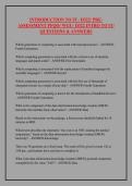
“Elements” (see Fig. 1.1), the great compilation produced by Euclid of
Alexandria in Ptolemaic Egypt circa 300 BC, established a unique logical
structure for mathematics whereby every mathematical theory is built upon
elementary axioms and definitions for which propositions and proofs follow.
Theories in physics also take a similar structure. For example, classical
mechanics is based on Sir Isaac Newton’s three laws of motion. Called
“laws”, they are in fact elementary hypotheses—that is, axioms. While this
may seem a remarkably different custom in physics compared to
Fig. 1.1 A fragment of Euclid’s Elements on part of the Oxyrhynchus papyri located at
the Uni- versity of Pennsylvania. Courtesy of WikiMedia Commons
Supplementary Information The online version contains supplementary material
available at https://doi.org/10.1007/978-3-030-91214-7_1.
© The Author(s), under exclusive license to Springer Nature Switzerland AG 2022 1
M.-S. Choi, A Quantum Computation
Workbook, https://doi.org/10.1007/978-3-
030-91214-7_1
,2 1 The Postulates of Quantum
Mechanics
its mathematical counterpart, it should not be surprising to refer to
assumptions as laws or principles because they provide physical theories
with logical foundation and are functional to determine whether Nature has
been described properly or they have a mere existence as an intellectual
framework. After all, the true value of a physical science is to understand
Nature.
Embracing the wave-particle duality and the complementarity principle,
quantum mechanics has been founded on the three fundamental
postulates. The founders of quantum mechanics could have been more
ambitious to call these laws instead of plain postulates, but each of these
three defies our intuition to such an extent that “postulates” sounds more
natural. As an overview, here are the fundamental postulates of quantum
mechanics:
Postulate 1 The quantum state of a system is completely described by a state
vector in the Hilbert space associated with the system.
Postulate 2 The time evolution of a closed quantum system is governed
by the Schrödinger equation.
Postulate 3 A physical quantity is described by an “observable”—a Hermitian
oper- ator. Upon measurement of the quantity, the outcome is one of the
eigenvalues of the observable and is determined probabilistically. Right after
the measurement, the state “collapses” to the eigenstate of the observable
corresponding to the measure- ment outcome.
In subsequent sections of this chapter, we detail the physical aspects of each
postulate and their relevance to quantum computing and quantum
information.
1.1 Quantum States
The first postulate indicates the mathematical description of the state of a
system. Recall that in classical mechanics, the state of a particle in motion is
described by the simple values of its position and momentum (or,
equivalently, velocity). In quantum mechanics, the description is formulated
at two different levels depending on the physical situation.
1.1.1 Pure States
Postulate 1 The quantum state of a closed system is completely described
by a state vector in the Hilbert space associated with the system.
The most common example of the state vector is a “wave function”—a member
of the Hilbert space of square integrable functions—originally put forward by
Schrödinger. Modern approaches associate an abstract vector space with
the system, and the spe- cific characters of the particular system are
,reflected in the choice of basis (see
,1.1 Quantum States 3
Appendix A.1). When the state is exactly known, the system is said to be in
its pure state, and the above description is comprehensive. However, in
many cases, it is difficult to know the exact state, and we thus need a more
general description to be discussed in the next subsection.
This postulate immediately raises a mind-blowing question: What is the
physi- cal meaning of the state vector or its components in a given basis
(or of the wave function)? Quantum mechanics has never offered a direct
physical meaning of the state vector. Born (1926) proposed a partial
resolution to the question and inspired the probabilistic interpretation of
quantum mechanics, as formulated in Postulate 3 concerning
measurement. This work awarded him the 1954 Nobel Prize in Physics.
Postulate 1 leaves another baffling question: Given a physical system, there
is no general prescription to figure out the Hilbert space associated with it.
While it is a rather technical question, it is nevertheless an important and
serious one when trying to describe a new system (or a yet-to-be-
understood system) quantum mechanically. For a qubit—an idealistic two-
level quantum system—the Hilbert space is two-
dimensional. A basis of two logical states |0 and |1 is assumed, and it is
called the
logical basis of the qubit.
Consider a group of two-level quantum systems, indicated by the symbol S .
E T [ UBI T S]
Di erent qubits can be specified by the flavor indices, the last of which has a special meaning
(see the documentation of Qubit ).
In[ ]:= { S[ 1, None] , S[ 2, None] }
S[ { 1, 2} , None]
Out[ ]= {S1, S2}
Out[ ]= {S1, S2}
The associated Hilbert space is two dimensional. For many functions dealing with qubits, the
final index ON E can be dropped.
In[ ]:= B S = AS I S [ S[ 1, ONE ] ]
BS = AS I S [ S[ 1] ]
Out[ ]= , 1 S1
Out[ ]= , 1 S1
For the e iciency reasons, the default value 0 of any qubit is removed from the data
structure. For a more intuitively appealing form with all default values, LogicalForm
can be used.
In[ ]:= LogicalForm [bs]
Out[ ]= 0 S1 , 1 S1
Each state in the logical basis can also be specified manually.
, 4 1 The Postulates of Quantum
Mechanics
In[ ]:= v ec = Ket [ S[ 1] 1, S[ 2] 0] ;
Logi cal For m[ vec, { S[ 1] , S[ 2] } ]
Out[ ]= 1 S1 0 S2
In[ ]:= v ec = Ket [ ] S[ 1{ , S[ 2{ } ] 1, 0} { ;
Logi cal For m[ vec, ] S[ 1{ , S[ 2{ } {
Out[ ]= 1 S1 0 S2
Ageneral quantum state of S[1,None] is a linear combination of the two basis states with two
complex coe icients c[0] and c[1] .
In[ ]:= Let [ Compl ex , c ]
vec = Ket [ S[ 1] 0] c[ 0] + Ket [ S[ 1] 1] c[ 1] ; vec /
/ Logi cal For m
Out[ ]= C 0 0S1 + C 1 1S1
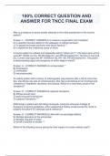
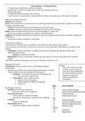
A two-dimensional state vector is often visualized as a point, called the
Bloch vector, on the Bloch sphere. The Bloch sphere is a geometrical
representation of a two-dimensional vector space. Any state vector |ψ is
expanded in the logical basis as
|ψ = |0 ψ0 + |1 ψ1 (ψ0, ψ1 ∈ C) . (1.1)
The normalization condition, |ψ0|2 + |ψ1|2 = 1, tells us that the state vector can
be expressed up to a global phase factor by
|ψ = |0 cos(θ/2) + |1 sin(θ/2)ei φ (1.2)
with θ and φ respectively specifying the magnitude and phase, of the
expansion coef- ficients (θ, φ ∈ R). The Bloch vector associated with the state
vector |ψ is defined by b = (sin θ cos φ, sin θ sin φ, cos θ). The Bloch vector can
equivalently be obtained in terms of the expectation values of the Pauli
operators, b = ( σ̂x , σ̂y , σ̂z ). Indeed, with |ψ in the form (1.2), one can show
that σ̂x = sin θ cos φ, σ̂y = sin θ sin φ, and σ̂z = cos θ . Therefore, any state
vector in a two-dimensional Hilbert space corresponds uniquely (up to a
global phase factor) to a point on the sphere with unit
radius, the Bloch sphere.
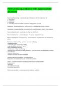
A two-dimensional pure state is represented by a point on the Bloch sphere. For example,
consider a pure state.
In[ ]:= v ec [ Ket ] = Sqr t ] 2= + I Ket ] S] 1= 1=;
vec / / Logi cal For m
Out[ ]= 1 S02 + 2 02
This visualize the state vector on a Bloch sphere. Bl ochVect or converts the state vector to a
three-dimensional vector. Bl ochSpher e is a shortcut for Gr aphi cs3D with an visualization of
the Bloch sphere.
1 The Postulates of Quantum Mechanics ................................................ 1
1.1 Quantum States .......................................................................... 2
1.1.1 Pure States ....................................................................... 2
1.1.2 Mixed States ..................................................................... 7
1.2 Time Evolution of Quantum States ............................................. 16
1.2.1 Unitary Dynamics............................................................ 17
1.2.2 Quantum Noisy Dynamics ............................................... 20
1.3 Measurements on Quantum States ............................................ 21
1.3.1 Projection Measurements ................................................ 21
1.3.2 Generalized Measurements............................................. 26
2 Quantum Computation: Overview ...................................................... 33
2.1 Single-Qubit Gates .................................................................... 34
2.1.1 Pauli Gates ..................................................................... 34
2.1.2 Hadamard Gate .............................................................. 39
2.1.3 Rotations ........................................................................ 42
2.2 Two-Qubit Gates ....................................................................... 46
2.2.1 CNOT, CZ, and SWAP................................................................ 46
2.2.2 Controlled-Unitary Gate................................................... 57
2.2.3 General Unitary Gate ...................................................... 63
2.3 Multi-Qubit Controlled Gates...................................................... 70
2.3.1 Gray Code ...................................................................... 71
2.3.2 Multi-Qubit Controlled-NOT ............................................. 73
2.4 Universal Quantum Computation ............................................... 79
2.5 Measurements .......................................................................... 81
3 Realizations of Quantum Computers 89
.3.1. . . . Quantum
. . . . . . . . . Bits
. . . . ...................... . . . . . . . . . . . . . . . . . . . . . . . . . . . . . . . 90
.3.2
. . . Dynamical Scheme . . . . . . . . . . . . . . . . . . . . . . . . . . . . . . . . . . . . . 92
. . . . 3.2.1 Implementation of Single-Qubit Gates . . . . . . . . . . . . . . . 93
.3.2.2
.. Implementation of CNOT . 99
............................
vii
,viii Contents
3.3 Geometric/Topological Scheme.................................................102
3.3.1 A Toy Model ...................................................................103
3.3.2 Geometric Phase ...........................................................109
3.4 Measurement-Based Scheme...................................................112
3.4.1 Single-Qubit Rotations ...................................................116
3.4.2 CNOT Gate ....................................................................119
3.4.3 Graph States..................................................................122
4 Quantum Algorithms.........................................................................127
4.1 Quantum Teleportation .............................................................128
4.1.1 Nonlocality in Entanglement ...........................................129
4.1.2 Implementation of Quantum Teleportation .......................132
4.2 Deutsch-Jozsa Algorithm & Variants ............................................. 136
4.2.1 Quantum Oracle.............................................................136
4.2.2 Deutsch-Jozsa Algorithm................................................142
4.2.3 Bernstein-Vazirani Algorithm ..........................................144
4.2.4 Simon’s Algorithm ..........................................................145
4.3 Quantum Fourier Transform (QFT) .......................................... 150
4.3.1 Definition and Physical Meaning .....................................150
4.3.2 Quantum Implementation ...............................................152
4.3.3 Semiclassical Implementation.........................................156
4.4 Quantum Phase Estimation (QPE) ............................................160
4.4.1 Definition........................................................................160
4.4.2 Implementation ..............................................................162
4.4.3 Accuracy ........................................................................165
4.4.4 Simulation of the von Neumann Measurement ................166
4.5 Applications..............................................................................167
4.5.1 The Period-Finding Algorithm .........................................168
4.5.2 The Order-Finding Algorithm ..........................................175
4.5.3 Quantum Factorization Algorithm ....................................177
4.5.4 Quantum Search Algorithm ............................................178
5 Quantum Decoherence.....................................................................189
5.1 How Does Decoherence Occur? ...............................................190
5.2 Quantum Operations ................................................................196
5.2.1 Kraus Representation.....................................................197
5.2.2 Choi Isomorphism ..........................................................206
5.2.3 Unitary Representation ...................................................209
5.2.4 Examples .......................................................................210
5.3 Measurements as Quantum Operations ....................................215
5.4 Quantum Master Equation ........................................................216
5.4.1 Derivation.......................................................................219
5.4.2 Examples .......................................................................220
5.4.3 Solution Methods ...........................................................223
5.4.4 Examples Revisited........................................................229
Contents ix
, 5.5 Distance Between Quantum States ...........................................234
5.5.1 Norms and Distances .....................................................234
5.5.2 Hilbert–Schmidt and Trace Norms ...................................236
5.5.3 Hilbert–Schmidt and Trace Distances ..............................241
5.5.4 Fidelity .......................................................................... 246
6 Quantum Error-Correction Codes......................................................257
6.1 Elementary Examples: Nine-Qubit Code ...................................258
6.1.1 Bit-Flip Errors .................................................................258
6.1.2 Phase-Flip Error............................................................ 261
6.1.3 Shor’s Nine-Qubit Code ..................................................263
6.2 Quantum Error Correction.........................................................268
6.2.1 Quantum Error-Correction Conditions .............................268
6.2.2 Discretization of Errors ...................................................270
6.3 Stabilizer Formalism .................................................................271
6.3.1 Pauli Group ....................................................................274
6.3.2 Properties of the Stabilizers ........................................... 279
6.3.3 Unitary Gates in Stabilizer Formalism .............................282
6.3.4 Clifford Group.................................................................283
6.3.5 Measurements in Stabilizer Formalism .......................... 290
6.3.6 Examples .......................................................................291
6.4 Stabilizer Codes .......................................................................297
6.4.1 Bit-Flip Code ..................................................................299
6.4.2 Phase-Flip Code ............................................................301
6.4.3 Nine-Qubit Code ............................................................302
6.4.4 Five-Qubit Code .............................................................305
6.5 Surface Codes .........................................................................309
6.5.1 Toric Codes....................................................................310
6.5.2 Planar Codes .................................................................314
6.5.3 Recovery Procedure.......................................................316
7 Quantum Information Theory ............................................................323
7.1 Shannon Entropy......................................................................324
7.1.1 Definition........................................................................324
7.1.2 Relative Entropy .............................................................326
7.1.3 Mutual Information .........................................................328
7.1.4 Data Compression .........................................................330
7.2 Von Neumann Entropy ..............................................................331
7.2.1 Definition........................................................................331
7.2.2 Relative Entropy .............................................................334
7.2.3 Quantum Mutual Information ..........................................337
7.3 Entanglement and Entropy........................................................338
7.3.1 What is Entanglement? ..................................................339
7.3.2 Separability Tests ............................................................... 339
7.3.3 Entanglement Distillation ............................................... 343
7.3.4 Entanglement Measures.................................................345
x Contents
,Appendix A: Linear Algebra ................................................................. 349
Appendix B: Superoperators................................................................... 373
Appendix C: Group Theory..................................................................... 395
Appendix D: Mathematica Application Q3 ............................................... 405
Appendix E: Integrated Compilation of Demonstrations ........................... 407
Appendix F: Solutions to Select Problems............................................... 409
Bibliography .................................................................................................... 425
Index............................................................................................................... 431
,Chapter 1
The Postulates of Quantum Mechanics
“Elements” (see Fig. 1.1), the great compilation produced by Euclid of
Alexandria in Ptolemaic Egypt circa 300 BC, established a unique logical
structure for mathematics whereby every mathematical theory is built upon
elementary axioms and definitions for which propositions and proofs follow.
Theories in physics also take a similar structure. For example, classical
mechanics is based on Sir Isaac Newton’s three laws of motion. Called
“laws”, they are in fact elementary hypotheses—that is, axioms. While this
may seem a remarkably different custom in physics compared to
Fig. 1.1 A fragment of Euclid’s Elements on part of the Oxyrhynchus papyri located at
the Uni- versity of Pennsylvania. Courtesy of WikiMedia Commons
Supplementary Information The online version contains supplementary material
available at https://doi.org/10.1007/978-3-030-91214-7_1.
© The Author(s), under exclusive license to Springer Nature Switzerland AG 2022 1
M.-S. Choi, A Quantum Computation
Workbook, https://doi.org/10.1007/978-3-
030-91214-7_1
,2 1 The Postulates of Quantum
Mechanics
its mathematical counterpart, it should not be surprising to refer to
assumptions as laws or principles because they provide physical theories
with logical foundation and are functional to determine whether Nature has
been described properly or they have a mere existence as an intellectual
framework. After all, the true value of a physical science is to understand
Nature.
Embracing the wave-particle duality and the complementarity principle,
quantum mechanics has been founded on the three fundamental
postulates. The founders of quantum mechanics could have been more
ambitious to call these laws instead of plain postulates, but each of these
three defies our intuition to such an extent that “postulates” sounds more
natural. As an overview, here are the fundamental postulates of quantum
mechanics:
Postulate 1 The quantum state of a system is completely described by a state
vector in the Hilbert space associated with the system.
Postulate 2 The time evolution of a closed quantum system is governed
by the Schrödinger equation.
Postulate 3 A physical quantity is described by an “observable”—a Hermitian
oper- ator. Upon measurement of the quantity, the outcome is one of the
eigenvalues of the observable and is determined probabilistically. Right after
the measurement, the state “collapses” to the eigenstate of the observable
corresponding to the measure- ment outcome.
In subsequent sections of this chapter, we detail the physical aspects of each
postulate and their relevance to quantum computing and quantum
information.
1.1 Quantum States
The first postulate indicates the mathematical description of the state of a
system. Recall that in classical mechanics, the state of a particle in motion is
described by the simple values of its position and momentum (or,
equivalently, velocity). In quantum mechanics, the description is formulated
at two different levels depending on the physical situation.
1.1.1 Pure States
Postulate 1 The quantum state of a closed system is completely described
by a state vector in the Hilbert space associated with the system.
The most common example of the state vector is a “wave function”—a member
of the Hilbert space of square integrable functions—originally put forward by
Schrödinger. Modern approaches associate an abstract vector space with
the system, and the spe- cific characters of the particular system are
,reflected in the choice of basis (see
,1.1 Quantum States 3
Appendix A.1). When the state is exactly known, the system is said to be in
its pure state, and the above description is comprehensive. However, in
many cases, it is difficult to know the exact state, and we thus need a more
general description to be discussed in the next subsection.
This postulate immediately raises a mind-blowing question: What is the
physi- cal meaning of the state vector or its components in a given basis
(or of the wave function)? Quantum mechanics has never offered a direct
physical meaning of the state vector. Born (1926) proposed a partial
resolution to the question and inspired the probabilistic interpretation of
quantum mechanics, as formulated in Postulate 3 concerning
measurement. This work awarded him the 1954 Nobel Prize in Physics.
Postulate 1 leaves another baffling question: Given a physical system, there
is no general prescription to figure out the Hilbert space associated with it.
While it is a rather technical question, it is nevertheless an important and
serious one when trying to describe a new system (or a yet-to-be-
understood system) quantum mechanically. For a qubit—an idealistic two-
level quantum system—the Hilbert space is two-
dimensional. A basis of two logical states |0 and |1 is assumed, and it is
called the
logical basis of the qubit.
Consider a group of two-level quantum systems, indicated by the symbol S .
E T [ UBI T S]
Di erent qubits can be specified by the flavor indices, the last of which has a special meaning
(see the documentation of Qubit ).
In[ ]:= { S[ 1, None] , S[ 2, None] }
S[ { 1, 2} , None]
Out[ ]= {S1, S2}
Out[ ]= {S1, S2}
The associated Hilbert space is two dimensional. For many functions dealing with qubits, the
final index ON E can be dropped.
In[ ]:= B S = AS I S [ S[ 1, ONE ] ]
BS = AS I S [ S[ 1] ]
Out[ ]= , 1 S1
Out[ ]= , 1 S1
For the e iciency reasons, the default value 0 of any qubit is removed from the data
structure. For a more intuitively appealing form with all default values, LogicalForm
can be used.
In[ ]:= LogicalForm [bs]
Out[ ]= 0 S1 , 1 S1
Each state in the logical basis can also be specified manually.
, 4 1 The Postulates of Quantum
Mechanics
In[ ]:= v ec = Ket [ S[ 1] 1, S[ 2] 0] ;
Logi cal For m[ vec, { S[ 1] , S[ 2] } ]
Out[ ]= 1 S1 0 S2
In[ ]:= v ec = Ket [ ] S[ 1{ , S[ 2{ } ] 1, 0} { ;
Logi cal For m[ vec, ] S[ 1{ , S[ 2{ } {
Out[ ]= 1 S1 0 S2
Ageneral quantum state of S[1,None] is a linear combination of the two basis states with two
complex coe icients c[0] and c[1] .
In[ ]:= Let [ Compl ex , c ]
vec = Ket [ S[ 1] 0] c[ 0] + Ket [ S[ 1] 1] c[ 1] ; vec /
/ Logi cal For m
Out[ ]= C 0 0S1 + C 1 1S1
A two-dimensional state vector is often visualized as a point, called the
Bloch vector, on the Bloch sphere. The Bloch sphere is a geometrical
representation of a two-dimensional vector space. Any state vector |ψ is
expanded in the logical basis as
|ψ = |0 ψ0 + |1 ψ1 (ψ0, ψ1 ∈ C) . (1.1)
The normalization condition, |ψ0|2 + |ψ1|2 = 1, tells us that the state vector can
be expressed up to a global phase factor by
|ψ = |0 cos(θ/2) + |1 sin(θ/2)ei φ (1.2)
with θ and φ respectively specifying the magnitude and phase, of the
expansion coef- ficients (θ, φ ∈ R). The Bloch vector associated with the state
vector |ψ is defined by b = (sin θ cos φ, sin θ sin φ, cos θ). The Bloch vector can
equivalently be obtained in terms of the expectation values of the Pauli
operators, b = ( σ̂x , σ̂y , σ̂z ). Indeed, with |ψ in the form (1.2), one can show
that σ̂x = sin θ cos φ, σ̂y = sin θ sin φ, and σ̂z = cos θ . Therefore, any state
vector in a two-dimensional Hilbert space corresponds uniquely (up to a
global phase factor) to a point on the sphere with unit
radius, the Bloch sphere.
A two-dimensional pure state is represented by a point on the Bloch sphere. For example,
consider a pure state.
In[ ]:= v ec [ Ket ] = Sqr t ] 2= + I Ket ] S] 1= 1=;
vec / / Logi cal For m
Out[ ]= 1 S02 + 2 02
This visualize the state vector on a Bloch sphere. Bl ochVect or converts the state vector to a
three-dimensional vector. Bl ochSpher e is a shortcut for Gr aphi cs3D with an visualization of
the Bloch sphere.