1
1 Basic concepts: atoms
1.1 The notation:
50
24
Cr
shows that the atomic number, Z, is 24 and the mass number for the isotope is 50.
Number of protons = Number of electrons = Z = 24
Number of neutrons = Mass number – Z = 50 – 24 = 26
For each isotope, Z = 24 and so there are 24 electrons and 24 protons.
For mass numbers 52, 53 and 54, there are 28, 29 and 30 neutrons, respectively.
1.2 ‘Monotopic’ means that the element possesses only one isotope. Examples other
See Appendix 5 in H&S than As include P, Na and Be.
1.3 (a) Al is monotopic, i.e. there is only one naturally occurring isotope.
Z = 13 Mass number = 27
Number of electrons = Number of protons = 13
Notation: Number of neutrons = 27 – 13 = 14
27 (b) Br (Z = 35) has 2 naturally occurring isotopes.
13 Al
Each isotope has 35 electrons and 35 protons.
79 81 For the isotope with mass number 79: number of neutrons = 79 – 35 = 44
35 Br 35 Br
For the isotope with mass number 81: number of neutrons = 81 – 35 = 46
54 56 57 58 (c) Fe (Z = 26) has 4 naturally occurring isotopes.
26 Fe 26 Fe 26 Fe 26 Fe
Each isotope has 26 electrons and 26 protons.
For the isotope with mass number 54: number of neutrons = 54 – 26 = 28
For the isotope with mass number 56: number of neutrons = 56 – 26 = 30
For the isotope with mass number 57: number of neutrons = 57 – 26 = 31
For the isotope with mass number 58: number of neutrons = 58 – 26 = 32
1.4 Assume that 3H can be ignored since abundance is so low; error introduced by this
assumption is negligible. The mass numbers of 1H and 2H are 1 and 2 respectively.
Let % 1H = x, and % 2H = 100 – x
Then:
x × 1 (100 − x ) × 2
A r = 1.008 = +
100 100
100.8 = x + 200 – 2 x
x = 99.2
This result gives 99.2 % 1H and 0.8 % 2H. The values do not agree with those in
Appendix 5 (99.985 % 1H and 0.015 % 2H) because we have used integral atomic
masses for the isotopes. The accurate masses (5 sig. fig.) are 1.0078 and 2.0141,
and if you work through the above calculation again, this gives 99.98 % 1H and
0.02 % 2H.
,2 Basic concepts: atoms
1.5 (a) Isotopic abundances: 32S 95.02 %, 33S 0.75 %, 34S 4.21 %, 36S 0.02 %. Relative
intensities of peaks containing these isotopes must reflect their relative abundances.
m/z = 256 is assigned to (32S)8 – the most abundant peak.
S m/z = 257 is assigned to (32S)7(33S).
S S m/z = 258 is assigned to (32S)6(33S)2 and (32S)7(34S).
m/z = 259 is assigned to (32S)6(33S)(34S).
S S
m/z = 260 is assigned to (32S)6(34S)2.
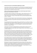
S S (b) The structure of S8 is shown in 1.1; the parent ion arises from S8. Fragmentation
S by S–S bond cleavage produces S7, S6, S5, S4 ... and gives lower mass peaks.
(1.1)
1.6 (a) c = λν
c
λ= c in m s–1, λ in m, ν in Hz (s–1)
ν
2.997 ×10⁸
λ= = 1.0 ×10− 4 m
3.0 ×10¹²
This lies in the far infrared region of the electromagnetic spectrum.
See Appendix 4 in H&S
(b)
2.997 ×10⁸
λ= = 3.0 ×10⁻¹⁰ m
1.0 ×10¹⁸
This lies in the X-ray region of the electromagnetic spectrum.
(c)
2.997 ×10⁸
λ= = 6.0 ×10⁻⁷ m
5.0 ×10¹⁴
This electromagnetic radiation is in the visible region.
1.7 Refer to Fig. 1.3 in H&S and the accompanying discussion.
Transitions to the level n = 1 belong to the Lyman series, therefore (a) and (e).
Transitions to the level n = 2 belong to the Balmer series, therefore (b) and (d).
Transitions to the level n = 2 belong to the Paschen series, therefore (c).
1.8 c
E = hν ν= Units: λ in m 450 nm = 450 × 10–9 m
λ
E = 4.41 × 10 −22 kJ
For the energy per mole, multiply by the Avogadro number:
E = 4.41 × 10 −22 × 6.022 × 10 23 = 266 kJ mol −1
1.9 Equation 1.4 in H&S is:
⎛ 1 1 ⎞
ν = R ⎜⎜ 2
− ⎟⎟
⎝2 n2 ⎠ where R = 1.097 × 10⁷ m–1
, Basic concepts: atoms 3
For n = 3:
⎛1 1⎞
ν = 1.097 × 10 7 ⎜ − ⎟ = 1.524 × 10 6 m −1
⎝4 9⎠
Convert m–1 to m, and then to nm (1 nm = 10–9 m) to obtain the wavelength in nm:
1
λ= × 10 9 = 656.2 nm (to 4 sig. fig.)
1 1.524 × 10 6
ν =
λ For n = 4:
⎛1 1⎞ −1
ν = 1.097 × 10 7 ⎜ − 6
⎟ = 2.057 × 10 m
⎝4 16 ⎠
1
λ= × 10 9 = 486.2 nm (to 4 sig. fig.)
2.057 × 10 6
Use the same method for n = 5, and n = 6, to obtain calculated values of λ of 434.1
nm and 410.2 nm respectively. Calculated values are consistent with observed lines
in the Balmer series.
1.10 The radii, rn, are found using eq. 1.8 in H&S, with values of n = 2 and n = 3.
where: ε0 = permittivity of a vacuum
ε 0h 2n 2
rn = h = Planck constant
πme e 2 me = electron rest mass
e = charge on an electron
For n = 2:
8.854 ×10 −12 × (6.626 × 10 −34 ) 2 × 2 2
rn = = 2.117 ×10 −10 m
π × 9.109 × 10 −31 × (1.602 × 10 −19 ) 2
or the radius may be quoted in pm: rn = 211.7 pm (1 pm = 10–12 m)
For n = 3:
8.854 × 10 −12 × (6.626 × 10 −34 ) 2 × 32
rn = = 4.764 × 10 −10 m
π × 9.109 ×10 −31 × (1.602 ×10 −19 ) 2
or: rn = 476.4 pm
1.11 As the value of n increases, (a) the energy of an ns orbital increases, and (b) the
size of the orbital increases.
1.12 (a) For the 6s orbital:
n = 6, l = 0, ml = 0
(b) Each of the five 4d orbitals has a unique set of quantum numbers:
n = 4, l = 2, ml = –2
n = 4, l = 2, ml = –1
n = 4, l = 2, ml = 0
n = 4, l = 2, ml = 1
n = 4, l = 2, ml = 2
1.13 (a) Principal quantum number = n. Each of the three 4p orbitals has a value of
n = 4.
, 4 Basic concepts: atoms
(b) For any np orbital, the orbital quantum number l = 1. Therefore the three 4p
orbitals have the same value of l.
(c) Each 4p orbital has a unique value of the magnetic quantum number, ml.
For the three 4p orbitals, the sets of quantum numbers are:
n = 4, l = 1, ml = –1
n = 4, l = 1, ml = 0
n = 4, l = 1, ml = 1
1.14 For information on radial nodes, see Figs. 1.7, 1.8 and 1.13 and accompanying
discussion in H&S. Radial nodes follow the trend shown below:
n 1 2 3 4 5 6
s 0 1 2 3 4 5
p 0 1 2 3 4
d 0 1 2 3
f 0 1 2
(a) A 2s orbital has 1 radial node.
(b) A 4s orbital has 3 radial nodes.
(c) A 3p orbital has 1 radial node.
(d) A 5d orbital has 2 radial nodes.
(e) A 1s orbital has no radial nodes.
(f) A 4p orbital has 2 radial nodes.
1.15 (a) Figure 1.5a in H&S shows a plot of R(r) against r for the 1s orbital of hydrogen.
An s orbital has a finite value of R(r) at the nucleus. Figure 1.7 in H&S shows a
plot of the radial distribution function, 4πr2R(r)2, against r for the hydrogen 1s
orbital; at the nucleus, the function is zero. The maximum value of 4πr2R(r)2 for
the 1s curve in Fig. 1.7 in H&S corresponds to the value of r at which the electron
has the highest probability of being found.
(b) For the 4s orbital of hydrogen, a plot of R(r) against r has both positive and
negative values of R(r); it has a positive value at r = 0 (i.e. at the nucleus). The 4s
orbital has 3 radial nodes; these are the three points at which the curve crosses the
axis along which r is plotted. Values of 4πr2R(r)2 are always greater or equal to
zero. A plot of 4πr2R(r)2 against r for the hydrogen 4s orbital has four points at
which the function is zero: at r = 0 and at three points corresponding to the radial
nodes.
(c) Figure 1.6 in H&S shows a plot of R(r) against r for the hydrogen 3p orbital. At
r = 0, R(r) = 0. The curve crosses the r axis once, and the function has both positive
and negative values. Figure. 1.8 in H&S shows a plot of 4πr2R(r)2 against r for the
3p orbital of hydrogen. The curve shows that the orbital has one radial node. Values
of 4πr2R(r)2 are always greater than or equal to zero.
1.16 Each orbital is defined by a set of three quantum numbers: n, l and ml.
(a) 1s: n = 1 l = 0 ... (n – 1), so only l = 0 is possible;
ml = +l, +(l – 1) ... 0 ... –(l – 1), –l , but since l = 0, only ml = 0 is possible.
Therefore, the set of quantum numbers that defines the 1s orbital is:
n = 1, l = 0, ml = 0.
1 Basic concepts: atoms
1.1 The notation:
50
24
Cr
shows that the atomic number, Z, is 24 and the mass number for the isotope is 50.
Number of protons = Number of electrons = Z = 24
Number of neutrons = Mass number – Z = 50 – 24 = 26
For each isotope, Z = 24 and so there are 24 electrons and 24 protons.
For mass numbers 52, 53 and 54, there are 28, 29 and 30 neutrons, respectively.
1.2 ‘Monotopic’ means that the element possesses only one isotope. Examples other
See Appendix 5 in H&S than As include P, Na and Be.
1.3 (a) Al is monotopic, i.e. there is only one naturally occurring isotope.
Z = 13 Mass number = 27
Number of electrons = Number of protons = 13
Notation: Number of neutrons = 27 – 13 = 14
27 (b) Br (Z = 35) has 2 naturally occurring isotopes.
13 Al
Each isotope has 35 electrons and 35 protons.
79 81 For the isotope with mass number 79: number of neutrons = 79 – 35 = 44
35 Br 35 Br
For the isotope with mass number 81: number of neutrons = 81 – 35 = 46
54 56 57 58 (c) Fe (Z = 26) has 4 naturally occurring isotopes.
26 Fe 26 Fe 26 Fe 26 Fe
Each isotope has 26 electrons and 26 protons.
For the isotope with mass number 54: number of neutrons = 54 – 26 = 28
For the isotope with mass number 56: number of neutrons = 56 – 26 = 30
For the isotope with mass number 57: number of neutrons = 57 – 26 = 31
For the isotope with mass number 58: number of neutrons = 58 – 26 = 32
1.4 Assume that 3H can be ignored since abundance is so low; error introduced by this
assumption is negligible. The mass numbers of 1H and 2H are 1 and 2 respectively.
Let % 1H = x, and % 2H = 100 – x
Then:
x × 1 (100 − x ) × 2
A r = 1.008 = +
100 100
100.8 = x + 200 – 2 x
x = 99.2
This result gives 99.2 % 1H and 0.8 % 2H. The values do not agree with those in
Appendix 5 (99.985 % 1H and 0.015 % 2H) because we have used integral atomic
masses for the isotopes. The accurate masses (5 sig. fig.) are 1.0078 and 2.0141,
and if you work through the above calculation again, this gives 99.98 % 1H and
0.02 % 2H.
,2 Basic concepts: atoms
1.5 (a) Isotopic abundances: 32S 95.02 %, 33S 0.75 %, 34S 4.21 %, 36S 0.02 %. Relative
intensities of peaks containing these isotopes must reflect their relative abundances.
m/z = 256 is assigned to (32S)8 – the most abundant peak.
S m/z = 257 is assigned to (32S)7(33S).
S S m/z = 258 is assigned to (32S)6(33S)2 and (32S)7(34S).
m/z = 259 is assigned to (32S)6(33S)(34S).
S S
m/z = 260 is assigned to (32S)6(34S)2.
S S (b) The structure of S8 is shown in 1.1; the parent ion arises from S8. Fragmentation
S by S–S bond cleavage produces S7, S6, S5, S4 ... and gives lower mass peaks.
(1.1)
1.6 (a) c = λν
c
λ= c in m s–1, λ in m, ν in Hz (s–1)
ν
2.997 ×10⁸
λ= = 1.0 ×10− 4 m
3.0 ×10¹²
This lies in the far infrared region of the electromagnetic spectrum.
See Appendix 4 in H&S
(b)
2.997 ×10⁸
λ= = 3.0 ×10⁻¹⁰ m
1.0 ×10¹⁸
This lies in the X-ray region of the electromagnetic spectrum.
(c)
2.997 ×10⁸
λ= = 6.0 ×10⁻⁷ m
5.0 ×10¹⁴
This electromagnetic radiation is in the visible region.
1.7 Refer to Fig. 1.3 in H&S and the accompanying discussion.
Transitions to the level n = 1 belong to the Lyman series, therefore (a) and (e).
Transitions to the level n = 2 belong to the Balmer series, therefore (b) and (d).
Transitions to the level n = 2 belong to the Paschen series, therefore (c).
1.8 c
E = hν ν= Units: λ in m 450 nm = 450 × 10–9 m
λ
E = 4.41 × 10 −22 kJ
For the energy per mole, multiply by the Avogadro number:
E = 4.41 × 10 −22 × 6.022 × 10 23 = 266 kJ mol −1
1.9 Equation 1.4 in H&S is:
⎛ 1 1 ⎞
ν = R ⎜⎜ 2
− ⎟⎟
⎝2 n2 ⎠ where R = 1.097 × 10⁷ m–1
, Basic concepts: atoms 3
For n = 3:
⎛1 1⎞
ν = 1.097 × 10 7 ⎜ − ⎟ = 1.524 × 10 6 m −1
⎝4 9⎠
Convert m–1 to m, and then to nm (1 nm = 10–9 m) to obtain the wavelength in nm:
1
λ= × 10 9 = 656.2 nm (to 4 sig. fig.)
1 1.524 × 10 6
ν =
λ For n = 4:
⎛1 1⎞ −1
ν = 1.097 × 10 7 ⎜ − 6
⎟ = 2.057 × 10 m
⎝4 16 ⎠
1
λ= × 10 9 = 486.2 nm (to 4 sig. fig.)
2.057 × 10 6
Use the same method for n = 5, and n = 6, to obtain calculated values of λ of 434.1
nm and 410.2 nm respectively. Calculated values are consistent with observed lines
in the Balmer series.
1.10 The radii, rn, are found using eq. 1.8 in H&S, with values of n = 2 and n = 3.
where: ε0 = permittivity of a vacuum
ε 0h 2n 2
rn = h = Planck constant
πme e 2 me = electron rest mass
e = charge on an electron
For n = 2:
8.854 ×10 −12 × (6.626 × 10 −34 ) 2 × 2 2
rn = = 2.117 ×10 −10 m
π × 9.109 × 10 −31 × (1.602 × 10 −19 ) 2
or the radius may be quoted in pm: rn = 211.7 pm (1 pm = 10–12 m)
For n = 3:
8.854 × 10 −12 × (6.626 × 10 −34 ) 2 × 32
rn = = 4.764 × 10 −10 m
π × 9.109 ×10 −31 × (1.602 ×10 −19 ) 2
or: rn = 476.4 pm
1.11 As the value of n increases, (a) the energy of an ns orbital increases, and (b) the
size of the orbital increases.
1.12 (a) For the 6s orbital:
n = 6, l = 0, ml = 0
(b) Each of the five 4d orbitals has a unique set of quantum numbers:
n = 4, l = 2, ml = –2
n = 4, l = 2, ml = –1
n = 4, l = 2, ml = 0
n = 4, l = 2, ml = 1
n = 4, l = 2, ml = 2
1.13 (a) Principal quantum number = n. Each of the three 4p orbitals has a value of
n = 4.
, 4 Basic concepts: atoms
(b) For any np orbital, the orbital quantum number l = 1. Therefore the three 4p
orbitals have the same value of l.
(c) Each 4p orbital has a unique value of the magnetic quantum number, ml.
For the three 4p orbitals, the sets of quantum numbers are:
n = 4, l = 1, ml = –1
n = 4, l = 1, ml = 0
n = 4, l = 1, ml = 1
1.14 For information on radial nodes, see Figs. 1.7, 1.8 and 1.13 and accompanying
discussion in H&S. Radial nodes follow the trend shown below:
n 1 2 3 4 5 6
s 0 1 2 3 4 5
p 0 1 2 3 4
d 0 1 2 3
f 0 1 2
(a) A 2s orbital has 1 radial node.
(b) A 4s orbital has 3 radial nodes.
(c) A 3p orbital has 1 radial node.
(d) A 5d orbital has 2 radial nodes.
(e) A 1s orbital has no radial nodes.
(f) A 4p orbital has 2 radial nodes.
1.15 (a) Figure 1.5a in H&S shows a plot of R(r) against r for the 1s orbital of hydrogen.
An s orbital has a finite value of R(r) at the nucleus. Figure 1.7 in H&S shows a
plot of the radial distribution function, 4πr2R(r)2, against r for the hydrogen 1s
orbital; at the nucleus, the function is zero. The maximum value of 4πr2R(r)2 for
the 1s curve in Fig. 1.7 in H&S corresponds to the value of r at which the electron
has the highest probability of being found.
(b) For the 4s orbital of hydrogen, a plot of R(r) against r has both positive and
negative values of R(r); it has a positive value at r = 0 (i.e. at the nucleus). The 4s
orbital has 3 radial nodes; these are the three points at which the curve crosses the
axis along which r is plotted. Values of 4πr2R(r)2 are always greater or equal to
zero. A plot of 4πr2R(r)2 against r for the hydrogen 4s orbital has four points at
which the function is zero: at r = 0 and at three points corresponding to the radial
nodes.
(c) Figure 1.6 in H&S shows a plot of R(r) against r for the hydrogen 3p orbital. At
r = 0, R(r) = 0. The curve crosses the r axis once, and the function has both positive
and negative values. Figure. 1.8 in H&S shows a plot of 4πr2R(r)2 against r for the
3p orbital of hydrogen. The curve shows that the orbital has one radial node. Values
of 4πr2R(r)2 are always greater than or equal to zero.
1.16 Each orbital is defined by a set of three quantum numbers: n, l and ml.
(a) 1s: n = 1 l = 0 ... (n – 1), so only l = 0 is possible;
ml = +l, +(l – 1) ... 0 ... –(l – 1), –l , but since l = 0, only ml = 0 is possible.
Therefore, the set of quantum numbers that defines the 1s orbital is:
n = 1, l = 0, ml = 0.