Tensorflow Cheat Sheet
Introduction to Tensorflow Example: Evaluating Tensors
import tensorflow as tf In TensorFlow 2.x, eager execution is enabled by de-
What is Tensorflow?
fault, which means operations are evaluated immedia-
TensorFlow is an open-source machine learning library scalar = tf.constant(7)
tely. In TensorFlow 1.x, you would have required a ses-
developed by the Google Brain team. Its name derives vector = tf.constant([7, 7])
matrix = tf.constant([[7, 7], [7, 7]]) sion to evaluate tensors.
from the operations which neural networks perform on
multi-dimensional data arrays, termed „tensors“. While tensor = tf.constant([1, 2, 3])
print(„Rank of scalar:“, tf.rank(scalar))
TensorFlow was originally designed for deep learning print(„Rank of vector:“, tf.rank(vector)) print(tensor.numpy()) # Converts tensor to a numpy array
tasks, it‘s versatile enough to be used for a wide variety print(„Rank of matrix:“, tf.rank(matrix)) and prints it
of other complex computational tasks.
Shape of Tensors Sources of Tensors
Key Features of TensorFlow The shape of a tensor defines how many elements are tf.zeros(): Creates a tensor with all elements set to zero.
Scalability: TensorFlow can run on a single CPU, on in each dimension. Using the shape attribute, you can
zero_tensor = tf.zeros(shape=(2, 3))
multiple CPUs/GPUs, and even on mobile devices. This retrieve the shape of any tensor.
makes it suitable for both research and production.
tensor = tf.constant([[1, 2, 3], [4, 5, 6]]) tf.ones(): Creates a tensor with all elements set to one.
Flexibility: TensorFlow isn‘t just for deep learning. You
can use it for traditional machine learning algorithms print(„Shape of tensor:“, tensor.shape)
one_tensor = tf.ones(shape=(2, 3))
or even general mathematical computations. Changing the Shape of Tensors
Visualization: With TensorBoard, TensorFlow offers a Sometimes, you might need to reshape a tensor. You
suite of visualization tools to analyze and visualize your Practice with Tensors
can use the reshape function for this.
model‘s structure and performance.
Addition
Production Ready: TensorFlow models can be easily tensor = tf.constant([[1, 2], [3, 4], [5, 6]])
You can add tensors using the + operator or the tf.add()
deployed to any platform with TensorFlow Serving, reshaped_tensor = tf.reshape(tensor, (2, 3))
print(„Reshaped tensor:\n“, reshaped_tensor) function.
TensorFlow Lite, and TensorFlow.js.
tensor1 = tf.constant([1, 2, 3])
Types of Tensors: Constant, Variable, Placeholder tensor2 = tf.constant([4, 5, 6])
Tensorflow Basics Constant: Immutable tensors whose values can‘t be result = tensor1 + tensor2 # or tf.add(tensor1, tensor2)
Tensor Basics changed. print(result.numpy())
In TensorFlow, data is represented as tensors. A tensor
is a generalization of vectors and matrices to potentially constant_tensor = tf.constant([1, 2, 3]) Multiplication (Element-wise)
higher dimensions, and it‘s the fundamental data struc- Element-wise multiplication can be performed using
Variable: Tensors whose values can change. They are ty- the * operator or the tf.multiply() function.
ture in TensorFlow.
pically used for weights and biases in a neural network.
tensor1 = tf.constant([1, 2, 3])
Rank of Tensors tensor2 = tf.constant([4, 5, 6])
variable_tensor = tf.Variable([1, 2, 3])
The rank of a tensor refers to the number of dimensions result = tensor1 * tensor2 # or tf.multiply(tensor1, tensor2)
it has. For instance: Placeholder: (Deprecated in TensorFlow 2.x) They were
print(result.numpy())
A scalar has rank 0. used to feed external data into a TensorFlow graph. In
A vector has rank 1. Matrix Multiplication
TensorFlow 2.x, this approach has been replaced by
A matrix has rank 2. For matrix multiplication, you can use the tf.matmul()
using tf.data for input pipelines.
And so on for higher dimensions. function or the @ operator in Python.
1
, Tensorflow Cheat Sheet
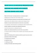
methods by which they do so. The versatility of Tensor- # Visualizing the data
matrix1 = tf.constant([[1, 2], [3, 4]]) plt.scatter(X_data, y_data, label=“Original Data“)
matrix2 = tf.constant([[5, 6], [7, 8]]) Flow lies in its comprehensive collection of tools and
plt.xlabel(„X“)
result = tf.matmul(matrix1, matrix2) # or matrix1 @ matrix2 algorithms that facilitate:
plt.ylabel(„y“)
print(result.numpy()) Data Preprocessing: Transforming raw data into a plt.legend()
format suitable for training. plt.show()
Broadcasting in TensorFlow Model Development: Defining the architecture and
Broadcasting allows TensorFlow to automatically ex- parameters of the model. From the plot, we can observe a linear relationship bet-
pand the dimensions of a smaller tensor to match the Training: Optimizing the model based on data. ween X_data and y_data.
shape of a larger tensor, making certain operations fea- Evaluation: Assessing the performance of the model.
sible. Deployment: Integrating the trained model into appli- Defining, Training, and Evaluating a Model
cations or services. With the data in place, let‘s define a simple linear re-
tensor = tf.constant([[1, 2, 3], [4, 5, 6]]) gression model using TensorFlow‘s Keras API.
scalar = tf.constant(2)
result = tensor * scalar # This multiplies every element in the # Defining the model
tensor by the scalar Linear Regression with Tensorflow model = tf.keras.Sequential()
print(result.numpy()) Linear Regression is a supervised learning algorithm model.add(tf.keras.layers.Dense(units=1, input_shape=[1]))
used to predict a continuous dependent variable based
In the example above, the scalar value 2 is „broadcast“ # Compile the model with loss and optimizer
on one or more independent variables. The goal is to fit model.compile(optimizer=‘sgd‘, loss=‘mean_squared_er-
to match the shape of the tensor, allowing element-wise the best line that accurately predicts the output values ror‘)
multiplication. within a range.
# Train the model
Setting up and Importing Necessary Libraries history = model.fit(X_data, y_data, epochs=100, verbose=0)
Tensorflow Core Learning Algorithms Before diving into linear regression, you need to ensure # Training for 100 epochs
that you have TensorFlow installed and then import the
TensorFlow provides implementations for a vast array # Predicting using the trained model
necessary libraries.
of machine learning algorithms, making it an ideal tool y_pred = model.predict(X_data)
for both classical machine learning and deep learning. # Install TensorFlow (if not done already)
# Visualizing original data and the regression line
# !pip install tensorflow
plt.scatter(X_data, y_data, label=“Original Data“)
Supervised Learning Algorithms: Linear Regression, # Importing necessary libraries plt.plot(X_data, y_pred, color=‘red‘, label=“Fitted Line“)
Logistic Regression, Support Vector Machines, etc. import tensorflow as tf plt.xlabel(„X“)
Unsupervised Learning Algorithms: K-Means Clus- import numpy as np plt.ylabel(„y“)
tering, Principal Component Analysis, etc. import matplotlib.pyplot as plt plt.legend()
Deep Learning Algorithms: Neural Networks, Con- plt.show()
volutional Neural Networks, Recurrent Neural Net- Loading and Inspecting Data
# Evaluating the model‘s loss on the data
works, etc. For this example, let‘s consider a simple dataset where
loss = model.evaluate(X_data, y_data, verbose=0)
Reinforcement Learning Algorithms: Q-Learning, we‘re trying to predict y values from x values. print(f “Mean Squared Error after training: {loss}“)
Deep Q-Networks, etc.
# Sample data
The red line in the plot represents the best-fit line our
Importance in Machine Learning X_data = np.array([1, 2, 3, 4, 5], dtype=float)
linear regression model has found. The Mean Squared
Machine learning revolves around the idea of teaching y_data = np.array([2, 4, 5.8, 8.1, 10.3], dtype=float)
Error (MSE) gives us a quantitative measure of how well
computers to learn from data, and algorithms are the our model fits the data: the lower the MSE, the better.
2
Introduction to Tensorflow Example: Evaluating Tensors
import tensorflow as tf In TensorFlow 2.x, eager execution is enabled by de-
What is Tensorflow?
fault, which means operations are evaluated immedia-
TensorFlow is an open-source machine learning library scalar = tf.constant(7)
tely. In TensorFlow 1.x, you would have required a ses-
developed by the Google Brain team. Its name derives vector = tf.constant([7, 7])
matrix = tf.constant([[7, 7], [7, 7]]) sion to evaluate tensors.
from the operations which neural networks perform on
multi-dimensional data arrays, termed „tensors“. While tensor = tf.constant([1, 2, 3])
print(„Rank of scalar:“, tf.rank(scalar))
TensorFlow was originally designed for deep learning print(„Rank of vector:“, tf.rank(vector)) print(tensor.numpy()) # Converts tensor to a numpy array
tasks, it‘s versatile enough to be used for a wide variety print(„Rank of matrix:“, tf.rank(matrix)) and prints it
of other complex computational tasks.
Shape of Tensors Sources of Tensors
Key Features of TensorFlow The shape of a tensor defines how many elements are tf.zeros(): Creates a tensor with all elements set to zero.
Scalability: TensorFlow can run on a single CPU, on in each dimension. Using the shape attribute, you can
zero_tensor = tf.zeros(shape=(2, 3))
multiple CPUs/GPUs, and even on mobile devices. This retrieve the shape of any tensor.
makes it suitable for both research and production.
tensor = tf.constant([[1, 2, 3], [4, 5, 6]]) tf.ones(): Creates a tensor with all elements set to one.
Flexibility: TensorFlow isn‘t just for deep learning. You
can use it for traditional machine learning algorithms print(„Shape of tensor:“, tensor.shape)
one_tensor = tf.ones(shape=(2, 3))
or even general mathematical computations. Changing the Shape of Tensors
Visualization: With TensorBoard, TensorFlow offers a Sometimes, you might need to reshape a tensor. You
suite of visualization tools to analyze and visualize your Practice with Tensors
can use the reshape function for this.
model‘s structure and performance.
Addition
Production Ready: TensorFlow models can be easily tensor = tf.constant([[1, 2], [3, 4], [5, 6]])
You can add tensors using the + operator or the tf.add()
deployed to any platform with TensorFlow Serving, reshaped_tensor = tf.reshape(tensor, (2, 3))
print(„Reshaped tensor:\n“, reshaped_tensor) function.
TensorFlow Lite, and TensorFlow.js.
tensor1 = tf.constant([1, 2, 3])
Types of Tensors: Constant, Variable, Placeholder tensor2 = tf.constant([4, 5, 6])
Tensorflow Basics Constant: Immutable tensors whose values can‘t be result = tensor1 + tensor2 # or tf.add(tensor1, tensor2)
Tensor Basics changed. print(result.numpy())
In TensorFlow, data is represented as tensors. A tensor
is a generalization of vectors and matrices to potentially constant_tensor = tf.constant([1, 2, 3]) Multiplication (Element-wise)
higher dimensions, and it‘s the fundamental data struc- Element-wise multiplication can be performed using
Variable: Tensors whose values can change. They are ty- the * operator or the tf.multiply() function.
ture in TensorFlow.
pically used for weights and biases in a neural network.
tensor1 = tf.constant([1, 2, 3])
Rank of Tensors tensor2 = tf.constant([4, 5, 6])
variable_tensor = tf.Variable([1, 2, 3])
The rank of a tensor refers to the number of dimensions result = tensor1 * tensor2 # or tf.multiply(tensor1, tensor2)
it has. For instance: Placeholder: (Deprecated in TensorFlow 2.x) They were
print(result.numpy())
A scalar has rank 0. used to feed external data into a TensorFlow graph. In
A vector has rank 1. Matrix Multiplication
TensorFlow 2.x, this approach has been replaced by
A matrix has rank 2. For matrix multiplication, you can use the tf.matmul()
using tf.data for input pipelines.
And so on for higher dimensions. function or the @ operator in Python.
1
, Tensorflow Cheat Sheet
methods by which they do so. The versatility of Tensor- # Visualizing the data
matrix1 = tf.constant([[1, 2], [3, 4]]) plt.scatter(X_data, y_data, label=“Original Data“)
matrix2 = tf.constant([[5, 6], [7, 8]]) Flow lies in its comprehensive collection of tools and
plt.xlabel(„X“)
result = tf.matmul(matrix1, matrix2) # or matrix1 @ matrix2 algorithms that facilitate:
plt.ylabel(„y“)
print(result.numpy()) Data Preprocessing: Transforming raw data into a plt.legend()
format suitable for training. plt.show()
Broadcasting in TensorFlow Model Development: Defining the architecture and
Broadcasting allows TensorFlow to automatically ex- parameters of the model. From the plot, we can observe a linear relationship bet-
pand the dimensions of a smaller tensor to match the Training: Optimizing the model based on data. ween X_data and y_data.
shape of a larger tensor, making certain operations fea- Evaluation: Assessing the performance of the model.
sible. Deployment: Integrating the trained model into appli- Defining, Training, and Evaluating a Model
cations or services. With the data in place, let‘s define a simple linear re-
tensor = tf.constant([[1, 2, 3], [4, 5, 6]]) gression model using TensorFlow‘s Keras API.
scalar = tf.constant(2)
result = tensor * scalar # This multiplies every element in the # Defining the model
tensor by the scalar Linear Regression with Tensorflow model = tf.keras.Sequential()
print(result.numpy()) Linear Regression is a supervised learning algorithm model.add(tf.keras.layers.Dense(units=1, input_shape=[1]))
used to predict a continuous dependent variable based
In the example above, the scalar value 2 is „broadcast“ # Compile the model with loss and optimizer
on one or more independent variables. The goal is to fit model.compile(optimizer=‘sgd‘, loss=‘mean_squared_er-
to match the shape of the tensor, allowing element-wise the best line that accurately predicts the output values ror‘)
multiplication. within a range.
# Train the model
Setting up and Importing Necessary Libraries history = model.fit(X_data, y_data, epochs=100, verbose=0)
Tensorflow Core Learning Algorithms Before diving into linear regression, you need to ensure # Training for 100 epochs
that you have TensorFlow installed and then import the
TensorFlow provides implementations for a vast array # Predicting using the trained model
necessary libraries.
of machine learning algorithms, making it an ideal tool y_pred = model.predict(X_data)
for both classical machine learning and deep learning. # Install TensorFlow (if not done already)
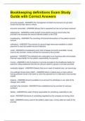
# Visualizing original data and the regression line
# !pip install tensorflow
plt.scatter(X_data, y_data, label=“Original Data“)
Supervised Learning Algorithms: Linear Regression, # Importing necessary libraries plt.plot(X_data, y_pred, color=‘red‘, label=“Fitted Line“)
Logistic Regression, Support Vector Machines, etc. import tensorflow as tf plt.xlabel(„X“)
Unsupervised Learning Algorithms: K-Means Clus- import numpy as np plt.ylabel(„y“)
tering, Principal Component Analysis, etc. import matplotlib.pyplot as plt plt.legend()
Deep Learning Algorithms: Neural Networks, Con- plt.show()
volutional Neural Networks, Recurrent Neural Net- Loading and Inspecting Data
# Evaluating the model‘s loss on the data
works, etc. For this example, let‘s consider a simple dataset where
loss = model.evaluate(X_data, y_data, verbose=0)
Reinforcement Learning Algorithms: Q-Learning, we‘re trying to predict y values from x values. print(f “Mean Squared Error after training: {loss}“)
Deep Q-Networks, etc.
# Sample data
The red line in the plot represents the best-fit line our
Importance in Machine Learning X_data = np.array([1, 2, 3, 4, 5], dtype=float)
linear regression model has found. The Mean Squared
Machine learning revolves around the idea of teaching y_data = np.array([2, 4, 5.8, 8.1, 10.3], dtype=float)
Error (MSE) gives us a quantitative measure of how well
computers to learn from data, and algorithms are the our model fits the data: the lower the MSE, the better.
2