Statistic 2 notes
Lecture 2:
Statistics 1: Differences between 2 groups.
Statistics 2: Differences between > 2 groups or relationships between variables.
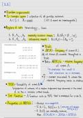
Contingency table/ cross table: Ways of looking at the table:
1. Marginal distribution:
- It gives the probabilities of various values of the variables in the
subset without reference to the values of the other variables.
Sum of the original random variables.
- The marginal distribution tells you the probability of a single
random variable without considering the others.
- For each row- or column total: Nkj / N
- Collection of these proportions for a variable is the marginal distribution of this variable.
- Sum of total for a variable = 1 or 100%.
2. Conditional distribution:
- Describes the probability that a random variable after
observing another random variable.
- It gives the probability distribution of one random variable,
given that another variable has a fixed value. It shows how
one variable behaves when the other is known or fixed.
- Calculate row- or column proportions.
- Set of these proportions for one variable is the conditional distribution for this variable.
- Every separate row (or column) adds up to 1 or 100%.
- Ignoring N.
3. Joint distribution:
- The probability distribution of all possible pairs of outputs of 2
random variables or each combination and not variation.
- For each cell: Nij / N.
- Collection of these proportions is the joint distribution of these 2 variables.
- Sum of all cells= 1 (or 100%).
When to use?
- Marinal distribution: What is the distribution of a single variable, ignoring others?
- Conditional distribution: Relationship? Focuses on 1 variable under the condition that
another is fixed.
- Joint distribution: Comparison between tables? Focusses on the combined behavior of 2 or
more variables.
,But: Hidden variables.
➢ Contingency table cannot contain more than 2 variables/dimensions.
➢ Are there hidden variables: Other variables can influence the variable in the table.
➢ “Simpson paradox”
- Nominal or ordinal hidden variable which influence the relationship.
- Aggregating groups can lead to a reserve relationship.
- Including hidden variables can lead to a reserve relationship.
Absolute numbers → Can be problematic to compare → add % (gives more information) → But still
need for a formal test: Chi-Square test.
When to choose the Chi-Square test?
- Differences between groups/ comparing groups (more than 2).
- Relationships between nominal/ ordinal variables: Testing independence of 2 nominal or
ordinal variables.
- Normal distribution is irrelevant since the test is based on categorical values.
Requirements Chi-Square test:
- Independent cases (assumption)
- Expected count per cell: For max. 20% of the cells: Lower than 5.
- For no cell: Lower than 1
But: Not meeting the requirements? → Adjust the data by combining categories.
- Reduce the number of columns, rows or categories= less variation.
- Not always the option and suitable→ how many cases does it impact?
1. Null hypothesis Chi-Square test:
➢ About the population, never about the sample.
➢ One specific situation: No difference, no relationship.
- In the population no relationship between variables.
- In the population, the variables are independent from one another.
- In the population, no difference in the distribution between groups.
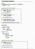
2. Calculating expected values.
Data= Observed number of cases per cell.
Fit= expected number/count of cases per cell based on the
H0, so when there is no relationship. But how to know?
Residual= Data (observed) – Fit (expected) for every cell: So
how var from the absolute zero?
Large difference between expected and actual: Relationship?
Because the expected counts are based on H0, and without a
relationship! →Is your observed count different?
,3. The actual Chi-Square test:
Notes:
→Same calculation for every cell.
→Why exponent? To be sure that the differences
are positive.
→Df: (Rows-1) * (Columns-1): more
col/rows→more degrees of freedom →More
significance.
→𝜒 2 Does not means that you need to square it!
Just the test symbol.
→Total of the table: Sum!
4. Test results:
1. Chi-square statistic table with use of degrees of freedom gives the p-value.
Note: Sometimes interpolation needed.
Or
2. You know degrees of freedom Gives you the critical 𝜒 2 – value.
You know critical p-value (0.05)
3. P-value < 0.05?
5. Conclusion:
- p=0.000, so p < 0.05.
- Test result is significant.
- Reject H0.
- We may assume that there is a relationship between the variables (or we may assume there
is a difference between the groups).
Important:
→For χ 2 (Chi-Squared test):
- Asymmetric distribution.
- Theoretical two-tailed, but practical one-tailed, because of the exponent in the formula,
there a no negative outcomes.
Interpretation:
1. Relationship: Significance does not say anything about the direction of a relationship.
2. Causality: Significance does not say anything about the existence of a causal relationship.
3. Significance: Chi-Square sensitive for increasing number of n.
Another test:
➢ Chi-Square test: 2 nominal/ordinal variables.
➢ One sample Square test/ Goodness Of Fit: Compare distribution of nominal/ordinal variable
with test distribution (from theory or wider population).
- “Same as the single sample t/z-test, but categorical”→Main difference is the setting.
, 1. Null- hypothesis one sample Chi-Square test:
➢ About the population, never about the sample.
➢ One specific situation: No difference, no relationship.
- In the population the distribution (of the data) is equal to the test distribution.
- Among the population of residents of the UK, the distribution of trust in the EU Parliament
equals to the distribution of trust in the UN.
2. Calculating expected values: Same as for the regular Chi-Square test.
Note: Mostly, the corresponding probability value in the test distribution is a percentage.
Example:
3. Test results & conclusion:
Degrees of freedom for the one-sample Chi-square test→Number of categories (k) -1.
Lecture 2:
Statistics 1: Differences between 2 groups.
Statistics 2: Differences between > 2 groups or relationships between variables.
Contingency table/ cross table: Ways of looking at the table:
1. Marginal distribution:
- It gives the probabilities of various values of the variables in the
subset without reference to the values of the other variables.
Sum of the original random variables.
- The marginal distribution tells you the probability of a single
random variable without considering the others.
- For each row- or column total: Nkj / N
- Collection of these proportions for a variable is the marginal distribution of this variable.
- Sum of total for a variable = 1 or 100%.
2. Conditional distribution:
- Describes the probability that a random variable after
observing another random variable.
- It gives the probability distribution of one random variable,
given that another variable has a fixed value. It shows how
one variable behaves when the other is known or fixed.
- Calculate row- or column proportions.
- Set of these proportions for one variable is the conditional distribution for this variable.
- Every separate row (or column) adds up to 1 or 100%.
- Ignoring N.
3. Joint distribution:
- The probability distribution of all possible pairs of outputs of 2
random variables or each combination and not variation.
- For each cell: Nij / N.
- Collection of these proportions is the joint distribution of these 2 variables.
- Sum of all cells= 1 (or 100%).
When to use?
- Marinal distribution: What is the distribution of a single variable, ignoring others?
- Conditional distribution: Relationship? Focuses on 1 variable under the condition that
another is fixed.
- Joint distribution: Comparison between tables? Focusses on the combined behavior of 2 or
more variables.
,But: Hidden variables.
➢ Contingency table cannot contain more than 2 variables/dimensions.
➢ Are there hidden variables: Other variables can influence the variable in the table.
➢ “Simpson paradox”
- Nominal or ordinal hidden variable which influence the relationship.
- Aggregating groups can lead to a reserve relationship.
- Including hidden variables can lead to a reserve relationship.
Absolute numbers → Can be problematic to compare → add % (gives more information) → But still
need for a formal test: Chi-Square test.
When to choose the Chi-Square test?
- Differences between groups/ comparing groups (more than 2).
- Relationships between nominal/ ordinal variables: Testing independence of 2 nominal or
ordinal variables.
- Normal distribution is irrelevant since the test is based on categorical values.
Requirements Chi-Square test:
- Independent cases (assumption)
- Expected count per cell: For max. 20% of the cells: Lower than 5.
- For no cell: Lower than 1
But: Not meeting the requirements? → Adjust the data by combining categories.
- Reduce the number of columns, rows or categories= less variation.
- Not always the option and suitable→ how many cases does it impact?
1. Null hypothesis Chi-Square test:
➢ About the population, never about the sample.
➢ One specific situation: No difference, no relationship.
- In the population no relationship between variables.
- In the population, the variables are independent from one another.
- In the population, no difference in the distribution between groups.
2. Calculating expected values.
Data= Observed number of cases per cell.
Fit= expected number/count of cases per cell based on the
H0, so when there is no relationship. But how to know?
Residual= Data (observed) – Fit (expected) for every cell: So
how var from the absolute zero?
Large difference between expected and actual: Relationship?
Because the expected counts are based on H0, and without a
relationship! →Is your observed count different?
,3. The actual Chi-Square test:
Notes:
→Same calculation for every cell.
→Why exponent? To be sure that the differences
are positive.
→Df: (Rows-1) * (Columns-1): more
col/rows→more degrees of freedom →More
significance.
→𝜒 2 Does not means that you need to square it!
Just the test symbol.
→Total of the table: Sum!
4. Test results:
1. Chi-square statistic table with use of degrees of freedom gives the p-value.
Note: Sometimes interpolation needed.
Or
2. You know degrees of freedom Gives you the critical 𝜒 2 – value.
You know critical p-value (0.05)
3. P-value < 0.05?
5. Conclusion:
- p=0.000, so p < 0.05.
- Test result is significant.
- Reject H0.
- We may assume that there is a relationship between the variables (or we may assume there
is a difference between the groups).
Important:
→For χ 2 (Chi-Squared test):
- Asymmetric distribution.
- Theoretical two-tailed, but practical one-tailed, because of the exponent in the formula,
there a no negative outcomes.
Interpretation:
1. Relationship: Significance does not say anything about the direction of a relationship.
2. Causality: Significance does not say anything about the existence of a causal relationship.
3. Significance: Chi-Square sensitive for increasing number of n.
Another test:
➢ Chi-Square test: 2 nominal/ordinal variables.
➢ One sample Square test/ Goodness Of Fit: Compare distribution of nominal/ordinal variable
with test distribution (from theory or wider population).
- “Same as the single sample t/z-test, but categorical”→Main difference is the setting.
, 1. Null- hypothesis one sample Chi-Square test:
➢ About the population, never about the sample.
➢ One specific situation: No difference, no relationship.
- In the population the distribution (of the data) is equal to the test distribution.
- Among the population of residents of the UK, the distribution of trust in the EU Parliament
equals to the distribution of trust in the UN.
2. Calculating expected values: Same as for the regular Chi-Square test.
Note: Mostly, the corresponding probability value in the test distribution is a percentage.
Example:
3. Test results & conclusion:
Degrees of freedom for the one-sample Chi-square test→Number of categories (k) -1.