Machine Learning
Cambiago Silvia Academic Year 2024-2025 Prof. Grégoire Montavon
DATA SCIENCE
Data science is defined in two ways: as a systematic study of data and as a data-driven approach
to scientific discovery, moving beyond traditional hypothesis-driven models.
While hypothesis-driven science depends on forming and testing specific questions, data
science capitalizes on high data availability, collecting and analyzing information without pre-
set hypotheses. This shift is supported by technological advances that make data collection
inexpensive and computational power abundant. Data science methods focus on identifying
patterns or correlations within large datasets, paving the way for new insights, hypothesis
generation, and feasibility assessments for predictive systems.
Data sources in data science are varied, including user data, biomedical information, historical
texts, and simulations. Often, these sources weren’t originally intended for scientific analysis
but can reveal unexpected patterns. For example, large repositories of GPS data show mobility
trends, while historical texts digitized for analysis provide unique cultural insights.
Additionally, simulation-generated data enables predictive modeling, supporting fields as
diverse as biomedical research and planetary science.
Machine learning is essential for managing high-dimensional data, which is difficult to
visualize or analyze manually. In addition to this, data can be high-dimensional (e.g. molecule),
hence not plottable in two dimensions. Techniques like dimensionality reduction simplify
complex data, making insights accessible and actionable. Biomedical applications, for instance,
apply methods such as T-SNE to identify cancer-related data clusters, while digital humanities
utilize machine learning to uncover visual and categorical correlations in historical
illustrations.
STORING, ACCESSING AND MANAGING DATA
Data consists of a collection of N instances where each instance can be represented as a vector
of d features. Such datasets can be stored in a two-dimensional array structure of size N ´ d
(like a NumPy array or a spreadsheet). Data typically comes with metadata, that describe what
the dataset is about, like what instances and features represent.
1
,Classical datasets are typically small enough to be stored on a single computer and to be loaded
into memory.
When instances are images, they may have different sizes and not fit in a tabular structure.
Same holds for other types of data such as speech or texts. The typical solution for these types
of data is to provide the dataset as a folder that contains composed of as many files as there are
instances. Subfolder structures may be added to organize instances according to their metadata.
In network datasets, data consists of a network of N instances, with connections between pairs
of related instances. Connections can be directed or undirected, weighted or not. Data can be
represented as an adjacency matrix (a tabular structure of size N × N) and can be stored in a
similar fashion as a classical dataset. Because the adjacency matrix is typically sparse (a node
is connected to less than 1% of remaining nodes on average), it is often preferrable to use a
sparse representation.
Relational databases are collection of tables, typically of two different types.
The first type of tables is similar to standard machine learning datasets, with each row
corresponding to an entity name (instance), and each column an attribute age category (feature).
The second type of table stores relations between instances of two different tables (e.g. which
customer bought which product). Data analysis of relational data may proceed either by:
µ Focusing on data from a single table;
µ Joining two or more tables via an INNER JOIN operation;
µ Operating directly on the relational structure using advanced data techniques.
Relational format allows to store data more compactly, since, for example, when there are many
relations between customer and products, there’s no need to restate multiple times the attributes
of the same customer or product.
It can happen that multiple small datasets
get aggregated in order to enable the
learning of more general and more
accurate models. For example, in the
figure it is shown an aggregation of omics
data from the TCGA corpus.
For aggregated datasets to be valuable, data coming from the multiple sources needs to be
homogenized, in terms of file formats, measurement units, and overall data model.
Furthermore, information that was implicit in the original datasets (e.g. use of a particular type
of sensor, data collected at a particular geographical location) need to be included in the
aggregated dataset, ideally in the form of additional features, or as metadata.
Data may have a level of heterogeneity such that there is no obvious data model that can be
used. In that case, the data model must be rebuilt from scratch using expert knowledge from
the field.
2
,Large datasets are datasets whose size is too large to be processed with classical techniques.
They are common when using high-throughput acquisition devices or when storing the output
of complex simulations. Advanced approaches are needed, making use of data parallelism and
synchronizing the model between the different machines.
DATA PREPROCESSING
Preprocessing is a critical stage in data science and machine learning where raw data is
transformed into a form suitable for analysis. Preprocessing varies significantly depending on
the data type, as each type of data requires specialized techniques to handle its properties:
µ Tabular data: tabular data given as csv files can be converted into an actual array via
the function numpy.genfromtxt. For Excel spreadsheets, the function
pandas.read_excel executes a similar conversion. Non-numerical variables may
either be discarded or converted to a numerical value (numpy.genfromtxt enables
the user to specify for a particular column how to the function transforming entries into
numerical values);
µ Relational data: operations such as INNER JOIN can be carried out with query language
such as SQL. In Python, sqlite3 can be used to create and access databases.
µ Image data: image datasets are typically provided using actual image files. Images can
be loaded in Python via PIL or cv2. Then, one can either use raw pixel values,
compute low-level features such as SIFT, or fed the image to a pretrained neural
network feature extractor such as VGG-16 or ResNet (available in Python via
torchvision);
µ Sound data: sound data is typically given as a sound file from which the waveform can
be extracted. In practice, it is common to convert the waveform into spectrograms
showing the frequency information at coarser time steps (e.g. using
scipy.signal.spectrogram);
µ Text data: text data is by nature non-numerical. It can be made numerical by converting
individual words to one-hot encodings if the vocabulary is small or to word embeddings
(e.g. via GloVe) if the vocabulary is large. Uninformative words such as ‘the’, ‘and’,
etc. may bias the data analysis. For a simple data analysis based on word frequencies,
it can be useful to preprocess the text by removing uninformative words.
VISUALIZATION
Visualization is an important component of data analysis, since it can provide evident insights
or suggest the application of certain models. It relies on the ability of the human to recognize
patterns in images or plots. Visualizations are typically 2D representations with colors, but 3D
or videos can also be applied. There are four basic categories of visualization techniques:
µ Array plots;
µ Histograms;
µ Scatter plots;
µ Graphs.
Most of the practically used visualizations can be seen as variants of these basic visualization
types.
3
, ARRAY PLOTS
In array plots, two-dimensional space is organized as a two-dimensional grid, where rows
represent instances and columns represent numerical features of the dataset.
Each element in the array is colored according to the
feature of the given instance, according to a color map.
Usually, the color is more intense in the instances where
the feature is more evident. A color bar is often shown next
to the plot. If the values are not colored, usually the data is
missing. Array plots can also be obtained for graph data by
visualizing the graph adjacency matrix.
Array plots have their own advantages and limitations. Among the strengths, lots of important
information about the structure of a dataset can be gathered from an array plot. Also, missing
values or lack of normalization are made extremely evident in this visualization.
On the other side, for large datasets it becomes overwhelming since it contains lots of
information. In addition to this, array plots do not give precise information on exact values
found in the table, the distribution of the values or correlations between features.
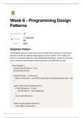
HISTOGRAMS
Histograms focus on a single numerical feature to extract more information about that feature.
Its values are not rendered as a color, but positions on the x-axis. The number of instances that
have that feature is given on the y-axis. If the distribution is heavily tailed, normalization can
be applied in order to make the visualization closer to a Gaussian distribution.
Histograms enable to extract a precise characterization of the distribution of feature values
considered individually, like mean and variance or the presence of outliers. But histograms do
not highlight possible correlations between features and are not suitable for high-dimensional
data.
4
Cambiago Silvia Academic Year 2024-2025 Prof. Grégoire Montavon
DATA SCIENCE
Data science is defined in two ways: as a systematic study of data and as a data-driven approach
to scientific discovery, moving beyond traditional hypothesis-driven models.
While hypothesis-driven science depends on forming and testing specific questions, data
science capitalizes on high data availability, collecting and analyzing information without pre-
set hypotheses. This shift is supported by technological advances that make data collection
inexpensive and computational power abundant. Data science methods focus on identifying
patterns or correlations within large datasets, paving the way for new insights, hypothesis
generation, and feasibility assessments for predictive systems.
Data sources in data science are varied, including user data, biomedical information, historical
texts, and simulations. Often, these sources weren’t originally intended for scientific analysis
but can reveal unexpected patterns. For example, large repositories of GPS data show mobility
trends, while historical texts digitized for analysis provide unique cultural insights.
Additionally, simulation-generated data enables predictive modeling, supporting fields as
diverse as biomedical research and planetary science.
Machine learning is essential for managing high-dimensional data, which is difficult to
visualize or analyze manually. In addition to this, data can be high-dimensional (e.g. molecule),
hence not plottable in two dimensions. Techniques like dimensionality reduction simplify
complex data, making insights accessible and actionable. Biomedical applications, for instance,
apply methods such as T-SNE to identify cancer-related data clusters, while digital humanities
utilize machine learning to uncover visual and categorical correlations in historical
illustrations.
STORING, ACCESSING AND MANAGING DATA
Data consists of a collection of N instances where each instance can be represented as a vector
of d features. Such datasets can be stored in a two-dimensional array structure of size N ´ d
(like a NumPy array or a spreadsheet). Data typically comes with metadata, that describe what
the dataset is about, like what instances and features represent.
1
,Classical datasets are typically small enough to be stored on a single computer and to be loaded
into memory.
When instances are images, they may have different sizes and not fit in a tabular structure.
Same holds for other types of data such as speech or texts. The typical solution for these types
of data is to provide the dataset as a folder that contains composed of as many files as there are
instances. Subfolder structures may be added to organize instances according to their metadata.
In network datasets, data consists of a network of N instances, with connections between pairs
of related instances. Connections can be directed or undirected, weighted or not. Data can be
represented as an adjacency matrix (a tabular structure of size N × N) and can be stored in a
similar fashion as a classical dataset. Because the adjacency matrix is typically sparse (a node
is connected to less than 1% of remaining nodes on average), it is often preferrable to use a
sparse representation.
Relational databases are collection of tables, typically of two different types.
The first type of tables is similar to standard machine learning datasets, with each row
corresponding to an entity name (instance), and each column an attribute age category (feature).
The second type of table stores relations between instances of two different tables (e.g. which
customer bought which product). Data analysis of relational data may proceed either by:
µ Focusing on data from a single table;
µ Joining two or more tables via an INNER JOIN operation;
µ Operating directly on the relational structure using advanced data techniques.
Relational format allows to store data more compactly, since, for example, when there are many
relations between customer and products, there’s no need to restate multiple times the attributes
of the same customer or product.
It can happen that multiple small datasets
get aggregated in order to enable the
learning of more general and more
accurate models. For example, in the
figure it is shown an aggregation of omics
data from the TCGA corpus.
For aggregated datasets to be valuable, data coming from the multiple sources needs to be
homogenized, in terms of file formats, measurement units, and overall data model.
Furthermore, information that was implicit in the original datasets (e.g. use of a particular type
of sensor, data collected at a particular geographical location) need to be included in the
aggregated dataset, ideally in the form of additional features, or as metadata.
Data may have a level of heterogeneity such that there is no obvious data model that can be
used. In that case, the data model must be rebuilt from scratch using expert knowledge from
the field.
2
,Large datasets are datasets whose size is too large to be processed with classical techniques.
They are common when using high-throughput acquisition devices or when storing the output
of complex simulations. Advanced approaches are needed, making use of data parallelism and
synchronizing the model between the different machines.
DATA PREPROCESSING
Preprocessing is a critical stage in data science and machine learning where raw data is
transformed into a form suitable for analysis. Preprocessing varies significantly depending on
the data type, as each type of data requires specialized techniques to handle its properties:
µ Tabular data: tabular data given as csv files can be converted into an actual array via
the function numpy.genfromtxt. For Excel spreadsheets, the function
pandas.read_excel executes a similar conversion. Non-numerical variables may
either be discarded or converted to a numerical value (numpy.genfromtxt enables
the user to specify for a particular column how to the function transforming entries into
numerical values);
µ Relational data: operations such as INNER JOIN can be carried out with query language
such as SQL. In Python, sqlite3 can be used to create and access databases.
µ Image data: image datasets are typically provided using actual image files. Images can
be loaded in Python via PIL or cv2. Then, one can either use raw pixel values,
compute low-level features such as SIFT, or fed the image to a pretrained neural
network feature extractor such as VGG-16 or ResNet (available in Python via
torchvision);
µ Sound data: sound data is typically given as a sound file from which the waveform can
be extracted. In practice, it is common to convert the waveform into spectrograms
showing the frequency information at coarser time steps (e.g. using
scipy.signal.spectrogram);
µ Text data: text data is by nature non-numerical. It can be made numerical by converting
individual words to one-hot encodings if the vocabulary is small or to word embeddings
(e.g. via GloVe) if the vocabulary is large. Uninformative words such as ‘the’, ‘and’,
etc. may bias the data analysis. For a simple data analysis based on word frequencies,
it can be useful to preprocess the text by removing uninformative words.
VISUALIZATION
Visualization is an important component of data analysis, since it can provide evident insights
or suggest the application of certain models. It relies on the ability of the human to recognize
patterns in images or plots. Visualizations are typically 2D representations with colors, but 3D
or videos can also be applied. There are four basic categories of visualization techniques:
µ Array plots;
µ Histograms;
µ Scatter plots;
µ Graphs.
Most of the practically used visualizations can be seen as variants of these basic visualization
types.
3
, ARRAY PLOTS
In array plots, two-dimensional space is organized as a two-dimensional grid, where rows
represent instances and columns represent numerical features of the dataset.
Each element in the array is colored according to the
feature of the given instance, according to a color map.
Usually, the color is more intense in the instances where
the feature is more evident. A color bar is often shown next
to the plot. If the values are not colored, usually the data is
missing. Array plots can also be obtained for graph data by
visualizing the graph adjacency matrix.
Array plots have their own advantages and limitations. Among the strengths, lots of important
information about the structure of a dataset can be gathered from an array plot. Also, missing
values or lack of normalization are made extremely evident in this visualization.
On the other side, for large datasets it becomes overwhelming since it contains lots of
information. In addition to this, array plots do not give precise information on exact values
found in the table, the distribution of the values or correlations between features.
HISTOGRAMS
Histograms focus on a single numerical feature to extract more information about that feature.
Its values are not rendered as a color, but positions on the x-axis. The number of instances that
have that feature is given on the y-axis. If the distribution is heavily tailed, normalization can
be applied in order to make the visualization closer to a Gaussian distribution.
Histograms enable to extract a precise characterization of the distribution of feature values
considered individually, like mean and variance or the presence of outliers. But histograms do
not highlight possible correlations between features and are not suitable for high-dimensional
data.
4