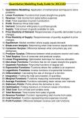
Quantitative Modelling Study Guide for DSC1520
1. Quantitative Modelling: Application of mathematical techniques to solve
problems.
2. Linear Functions: Functions that create straight-line graphs.
3. Revenue: Total income from sales before expenses.
4. Cost: Total expenses incurred in production.
5. Profit: Revenue minus total costs.
6. Demand: Consumer willingness to purchase goods.
7. Supply: Total amount of goods available for sale.
8. Price Elasticity of Demand: Responsiveness of quantity demanded to price
changes.
9. Price Elasticity of Supply: Responsiveness of quantity supplied to price
changes.
10. Equilibrium: Market condition where supply equals demand.
11. Break-even Analysis: Determining when total revenue equals total costs.
12. Consumer Surplus: Difference between what consumers pay and
willingness.
13. Producer Surplus: Difference between what producers receive and costs.
14. Total Surplus: Sum of consumer and producer surplus.
15. Linear Programming: Optimization technique for resource allocation.
16. Non-linear Functions: Functions that do not create straight-line graphs.
17. Quadratic Functions: Polynomial functions of degree two.
18. Exponential Functions: Functions where the variable is an exponent.
19. Logarithmic Functions: Inverse functions of exponential functions.
20. Differentiation: Calculating the rate of change of a function.
21. Integration: Finding the total accumulation of quantities.
22. Marginal Functions: Functions measuring incremental changes.
23. Average Functions: Functions calculating mean values over intervals.
24. Stationary Points: Points where the derivative is zero.
25. Optimisation: Finding maximum or minimum values of functions.
26. Total Cost: Sum of fixed and variable costs.
27. Total Revenue: Total income from sales of goods.
28. Revenue Function: Function representing total income from sales.
29. Cost Function: Function representing total expenses incurred.
30. Profit Function: Difference between revenue and cost functions.
, Quantitative Modelling Study Guide for DSC1520
31. Demand Function: Relationship between product price and quantity
demanded.
32. Supply Function: Relationship between product price and quantity supplied.
33. Elasticity: Measure of responsiveness in demand or supply.
34. Break-even Point: Point where total revenue equals total cost.
35. Complementary Goods: Goods that are consumed together.
36. Substitute Goods: Goods that can replace each other.
37. Taxes: Mandatory financial charges imposed by government.
38. Subsidies: Financial assistance to encourage production or consumption.
39. Hyperbolic Functions: Functions based on hyperbolas, analogous to
trigonometric functions.
40. Power Rule (Differentiation): Rule for finding derivatives of power functions.
41. Chain Rule: Method for differentiating composite functions.
42. Product Rule: Rule for differentiating products of functions.
43. Quotient Rule: Rule for differentiating quotients of functions.
44. Higher Derivatives: Derivatives of derivatives, indicating acceleration.
45. Production Functions: Functions that relate inputs to outputs in production.
46. Integration by Substitution: Method for simplifying integrals by changing
variables.
47. Definite Integral: Integral with specified upper and lower limits.
48. Total Functions: Functions that aggregate marginal changes over intervals.
49. Mathematical Modelling: Creating equations to represent real-life problems.
50. Learning Objectives: Key concepts to master in each chapter.
51. Worked Examples: Illustrations of how to solve specific problems.
52. Self-assessment Tests: Activities to evaluate understanding of material.
53. Basic Mathematics: Foundational skills assumed for module entry.
54. Variables: Symbols representing quantities in mathematical expressions.
55. Functions: Relationships between inputs and outputs.
56. Cubic Functions: Polynomial functions of degree three.
57. Composite Functions: Functions formed by combining two or more
functions.
58. Deterministic Models: Models with predictable outcomes based on inputs.
59. Stochastic Models: Models incorporating randomness and probability.
60. Physical Models: Tangible representations of concepts or systems.

