SPSS-sessie 1
1 Bivariate relations & simple regression
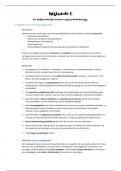
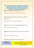
(1A) Make a scatter plot of skinfold thickness (LSKIN) (x-axis) and body mass (DEN)
(y-axis)
Graphs -> Scatter/Dot -> Simple scatter
1.120
1.100
1.080
1.060
den
1.040
1.020
1.000
0.980
0.80 1.00 1.20 1.40 1.60 1.80 2.00 2.20
lskin
(1B) Describe the relationship between skinfold and body mass:
• Linear or non-linear? -> linear
• Weak or strong? -> strong
• Positive or negative? -> negative
(1C) Perform a regression analysis to predict body mass (DEN) from skinfold
(LSKIN). What is the regression equation? What is the value of R2 and what does
this mean?
Analyze -> Regression -> Linear -> DV: DEN and IV: LSKIN (-> Statistics: R squared
change)
Regression equation general: DV = (intercept) + slope x IV
Equation specific: DEN = 1.163 (intercept) - .06LSKIN (slope x IV)
R2 = .72, so 72% of the variance in the body mass is explained by the skin fold
thickness.
(1D) Formulate the hypotheses concerning the regression coefficient. …
H0: 1 = 0
Ha: 1 0
(1E) What is your conclusion concerning this hypotheses?
In the coefficients table -> Sig. = < .001, so we can reject the H0.
, In APA-form: The regression coefficient of LSKIN is significant (t(90)=−15.23,p<.01).
From the b-value of LSKIN we can infer that an increase in skinfold thickness is
associated with a decrease in body mass (b=−.06).
(1F) Redo the analysis and save (use the Save option) the predicted values for body
mass. Look up the new variable in the data editor.
Analyze -> Regression -> Linear -> DV: DEN and IV: LSKIN (-> Statistics: R squared
change) -> Save: left column Predicted Values: Unstandardized
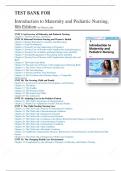
(1G) Make a scatter plot of skinfold thickness (LSKIN) (x-axis) and the predicted
values for body mass (y-axis). Compare this scatterplot to the one created in a.
Explain the difference between the two plot and include the term “residual” in this
explanation.
Same steps as 1A.
1.12000
Unstandardized Predicted
1.10000
1.08000
1.06000
Value
1.04000
1.02000
1.00000
0.98000
0.80 1.00 1.20 1.40 1.60 1.80 2.00 2.20
lskin
When you have regression analysis with only one predictor. You have a formula like:
Ypredicted= b0 + b1 X. The predicted values are thus a so-called linear
transformation of the predictor variable. Any linear transformation of a variable will be
perfectly correlated with the original variable. The conclusion is that your regression
,model predicts scores that are on a straight line, while “real data” are scattered
around this line and therefore there will be prediction errors (residuals).
2 Regression analysis: checking linearity assumption
Open the data file ‘MM02_060.SAV’, which is a fictive data set with four different
dependent variables Y1 to Y4 and four predictor variables X1 to X4. The goal is to
predict Y1 from X1, Y2 from X2, and so on.
(2A) Compute the correlations and regression coefficients for the 4 variable pairs
X1−Y1 through X4−Y4. What do you notice about these results?
Regression coefficients is b-value in table in
SPSS
Compute correlations: Analyze -> Correlate -
> Bivariate -> Fill in each pair (so X1 and Y1;
X2 and Y2 etc.)
Correlations for all four pairs: around .82
Compute regression coefficients: Analyze -> Regression -> Linear -> DV is Y-variable
of the pair, IV is the X-variable. Do this for each pair.
(2B) Make scatter plots (including regression lines) for each of the four X−Y variable
pairs.
Same way as 1A; DV on Y-axis (so Y1, Y2 etc.) and the IV on the X-axis (so X1, X2
etc.). The regression lines: double click on scatterplot and select Add line to fit total
Then you can choose which kind of line fits best.
Only for the relation between Y1 and X1, the (linear) regression equation is a good
and representative model. For the relation between X2 and Y2 a quadratic function
would be more representative; the relationship between X3 and Y3, and also X4 and
Y4 should be computed after removing the outlier (in case of X4 and Y4 the
correlation would be zero when the outlier would have been discarded).
(2C) Which of these regression lines provides a good description of the data?
See answer 2B.
(2D) Compute the average and the standard deviation for all eight variables (X1−X4,
and Y1−Y4). Make a note of these values. What do you notice? Could you have
expected this based on your earlier findings?
Analyze -> Descriptive statistics -> Descriptives -> Mean & Std. deviation
All the X-values have a mean of 9.00 and a SD of 3.32
All the Y-values have a mean of 7.50 and a SD of 2.03
I think you could have expected this, based on the findings at question 2A.
(2E) What important first step for all advanced types of data analysis is illustrated by
this exercise?
Graphically, explore the univariate (histograms) and bivariate (scatterplots)
distributions of your variables, before you conduct any statistical analysis.
, 3 Regression analysis: checking assumptions concerning residuals
Open the data file ‘STUDENT.SAV’. We will now try to predict the variable Weight
from the variable Height.
(3A) Run an analysis in SPSS to predict Weight from Height. Request a plot of the
standardized residuals (*ZRESID) versus the standardized predicted values of
Weight (*ZPRED)
Analyze -> Regression -> Linear -> DV: Weight & IV: Height -> Plots with *ZRED on
x-axis and *ZRESID on y-axis and check the boxes for Histogram and Normal
probability plot
(3B) Explain in what a residual is. What conditions should the residuals in this
analysis meet?
The residual or error equals Yobserved−Ypredicted
(3C) In the output, find the information you need to define the regression equation.
Write down your findings.
Outcome: weight
Intercept = -55.33 So, the equation: weight = -55.33 + 66.63 x height
Slope: 66.63
(3D) Now use the regression equation to predict the Weight of someone with a
Height of 1.75 m. How many kilograms could such a person be expected to weigh?
Weight = -55.33 + (66.63 x 1.75) = 61.27
(3E) What can you conclude based on the residuals plot? Write down your
conclusions.
The residual plot of the standardized predicted values (on the horizontal axis) against
the standardized residuals (on the vertical axis) can be used to check the following
assumptions of regression analysis:
1. Homogeneity of error variance across the entire range of predicted values
(homoscedasticity). This assumption is met when the points in the plot lie in
a horizontal band around the zero-line.
2. Normally distributed errors. The mean of the errors is zero by definition, but
we also check whether they are normally distributed around the mean of zero.
This is the case when most points are close to the zero-line and there are
approximately as many larger deviations above the zero-line, as there are
below it.
3. Linearity of the relation between Y and the predictor(s). This is the case when
the pattern of points around zero does not have a systematically deviant
shape (such as a curve or a wave)
In the current analysis we can conclude that
• the residuals have an approximately normal distribution
• the relation is approximately linear
• the error variance is approximately homogeneous; although for average
predicted values we see some large residuals. When we look at the histogram
of weight, we see that we have some outliers with respect to weight, which are
apparently not the tall
1 Bivariate relations & simple regression
(1A) Make a scatter plot of skinfold thickness (LSKIN) (x-axis) and body mass (DEN)
(y-axis)
Graphs -> Scatter/Dot -> Simple scatter
1.120
1.100
1.080
1.060
den
1.040
1.020
1.000
0.980
0.80 1.00 1.20 1.40 1.60 1.80 2.00 2.20
lskin
(1B) Describe the relationship between skinfold and body mass:
• Linear or non-linear? -> linear
• Weak or strong? -> strong
• Positive or negative? -> negative
(1C) Perform a regression analysis to predict body mass (DEN) from skinfold
(LSKIN). What is the regression equation? What is the value of R2 and what does
this mean?
Analyze -> Regression -> Linear -> DV: DEN and IV: LSKIN (-> Statistics: R squared
change)
Regression equation general: DV = (intercept) + slope x IV
Equation specific: DEN = 1.163 (intercept) - .06LSKIN (slope x IV)
R2 = .72, so 72% of the variance in the body mass is explained by the skin fold
thickness.
(1D) Formulate the hypotheses concerning the regression coefficient. …
H0: 1 = 0
Ha: 1 0
(1E) What is your conclusion concerning this hypotheses?
In the coefficients table -> Sig. = < .001, so we can reject the H0.
, In APA-form: The regression coefficient of LSKIN is significant (t(90)=−15.23,p<.01).
From the b-value of LSKIN we can infer that an increase in skinfold thickness is
associated with a decrease in body mass (b=−.06).
(1F) Redo the analysis and save (use the Save option) the predicted values for body
mass. Look up the new variable in the data editor.
Analyze -> Regression -> Linear -> DV: DEN and IV: LSKIN (-> Statistics: R squared
change) -> Save: left column Predicted Values: Unstandardized
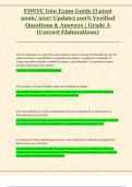
(1G) Make a scatter plot of skinfold thickness (LSKIN) (x-axis) and the predicted
values for body mass (y-axis). Compare this scatterplot to the one created in a.
Explain the difference between the two plot and include the term “residual” in this
explanation.
Same steps as 1A.
1.12000
Unstandardized Predicted
1.10000
1.08000
1.06000
Value
1.04000
1.02000
1.00000
0.98000
0.80 1.00 1.20 1.40 1.60 1.80 2.00 2.20
lskin
When you have regression analysis with only one predictor. You have a formula like:
Ypredicted= b0 + b1 X. The predicted values are thus a so-called linear
transformation of the predictor variable. Any linear transformation of a variable will be
perfectly correlated with the original variable. The conclusion is that your regression
,model predicts scores that are on a straight line, while “real data” are scattered
around this line and therefore there will be prediction errors (residuals).
2 Regression analysis: checking linearity assumption
Open the data file ‘MM02_060.SAV’, which is a fictive data set with four different
dependent variables Y1 to Y4 and four predictor variables X1 to X4. The goal is to
predict Y1 from X1, Y2 from X2, and so on.
(2A) Compute the correlations and regression coefficients for the 4 variable pairs
X1−Y1 through X4−Y4. What do you notice about these results?
Regression coefficients is b-value in table in
SPSS
Compute correlations: Analyze -> Correlate -
> Bivariate -> Fill in each pair (so X1 and Y1;
X2 and Y2 etc.)
Correlations for all four pairs: around .82
Compute regression coefficients: Analyze -> Regression -> Linear -> DV is Y-variable
of the pair, IV is the X-variable. Do this for each pair.
(2B) Make scatter plots (including regression lines) for each of the four X−Y variable
pairs.
Same way as 1A; DV on Y-axis (so Y1, Y2 etc.) and the IV on the X-axis (so X1, X2
etc.). The regression lines: double click on scatterplot and select Add line to fit total
Then you can choose which kind of line fits best.
Only for the relation between Y1 and X1, the (linear) regression equation is a good
and representative model. For the relation between X2 and Y2 a quadratic function
would be more representative; the relationship between X3 and Y3, and also X4 and
Y4 should be computed after removing the outlier (in case of X4 and Y4 the
correlation would be zero when the outlier would have been discarded).
(2C) Which of these regression lines provides a good description of the data?
See answer 2B.
(2D) Compute the average and the standard deviation for all eight variables (X1−X4,
and Y1−Y4). Make a note of these values. What do you notice? Could you have
expected this based on your earlier findings?
Analyze -> Descriptive statistics -> Descriptives -> Mean & Std. deviation
All the X-values have a mean of 9.00 and a SD of 3.32
All the Y-values have a mean of 7.50 and a SD of 2.03
I think you could have expected this, based on the findings at question 2A.
(2E) What important first step for all advanced types of data analysis is illustrated by
this exercise?
Graphically, explore the univariate (histograms) and bivariate (scatterplots)
distributions of your variables, before you conduct any statistical analysis.
, 3 Regression analysis: checking assumptions concerning residuals
Open the data file ‘STUDENT.SAV’. We will now try to predict the variable Weight
from the variable Height.
(3A) Run an analysis in SPSS to predict Weight from Height. Request a plot of the
standardized residuals (*ZRESID) versus the standardized predicted values of
Weight (*ZPRED)
Analyze -> Regression -> Linear -> DV: Weight & IV: Height -> Plots with *ZRED on
x-axis and *ZRESID on y-axis and check the boxes for Histogram and Normal
probability plot
(3B) Explain in what a residual is. What conditions should the residuals in this
analysis meet?
The residual or error equals Yobserved−Ypredicted
(3C) In the output, find the information you need to define the regression equation.
Write down your findings.
Outcome: weight
Intercept = -55.33 So, the equation: weight = -55.33 + 66.63 x height
Slope: 66.63
(3D) Now use the regression equation to predict the Weight of someone with a
Height of 1.75 m. How many kilograms could such a person be expected to weigh?
Weight = -55.33 + (66.63 x 1.75) = 61.27
(3E) What can you conclude based on the residuals plot? Write down your
conclusions.
The residual plot of the standardized predicted values (on the horizontal axis) against
the standardized residuals (on the vertical axis) can be used to check the following
assumptions of regression analysis:
1. Homogeneity of error variance across the entire range of predicted values
(homoscedasticity). This assumption is met when the points in the plot lie in
a horizontal band around the zero-line.
2. Normally distributed errors. The mean of the errors is zero by definition, but
we also check whether they are normally distributed around the mean of zero.
This is the case when most points are close to the zero-line and there are
approximately as many larger deviations above the zero-line, as there are
below it.
3. Linearity of the relation between Y and the predictor(s). This is the case when
the pattern of points around zero does not have a systematically deviant
shape (such as a curve or a wave)
In the current analysis we can conclude that
• the residuals have an approximately normal distribution
• the relation is approximately linear
• the error variance is approximately homogeneous; although for average
predicted values we see some large residuals. When we look at the histogram
of weight, we see that we have some outliers with respect to weight, which are
apparently not the tall